The whole of one-dimensional motion, one figure at a time.
Kinematics is the language you use to say what a body is doing before you ask why it does it. This page walks the whole of that language in order — motion diagrams, position, displacement, vectors, graphs, acceleration, and free fall — one figure at a time. Read it top to bottom the first time. After that, use the jump links to go straight to the thing you have forgotten.
This walkthrough covers one-dimensional motion. Projectile and two-dimensional motion — also part of A.1 — are not covered here; use the A.1 topic page for video support and worksheets on those.
Before any equation, you need a way of drawing motion that strips out everything irrelevant. That is what a motion diagram does.
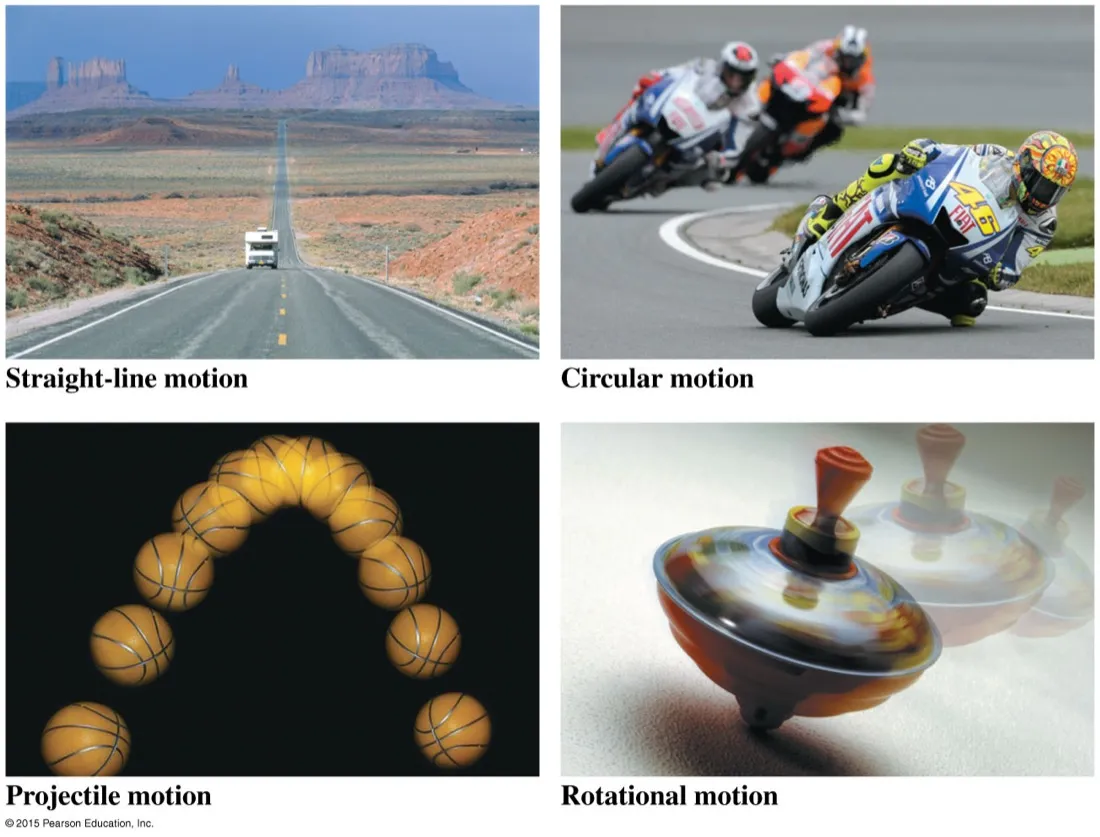
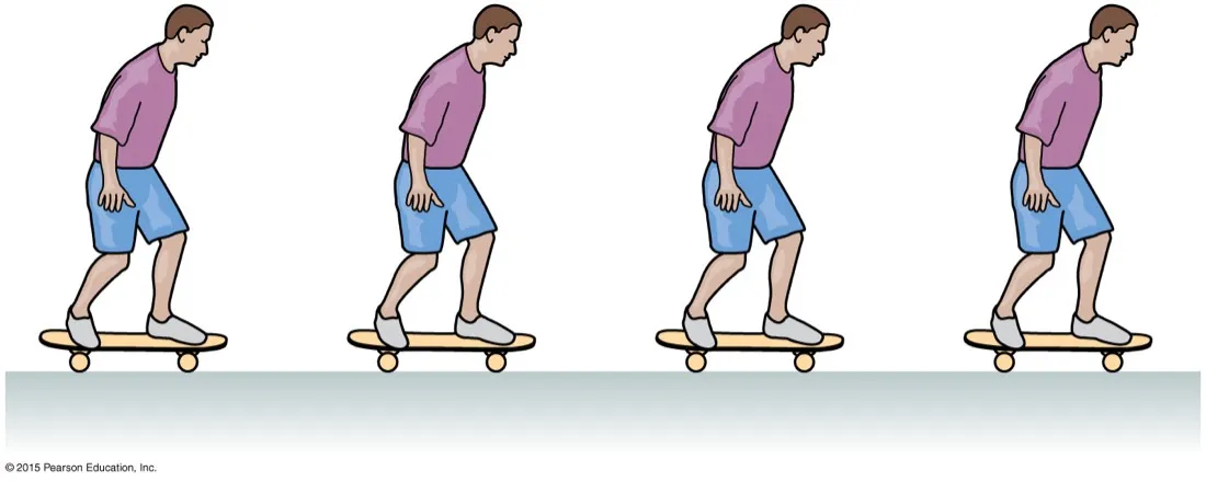
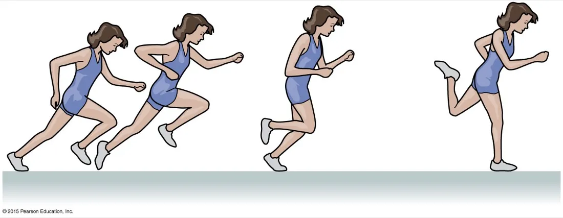
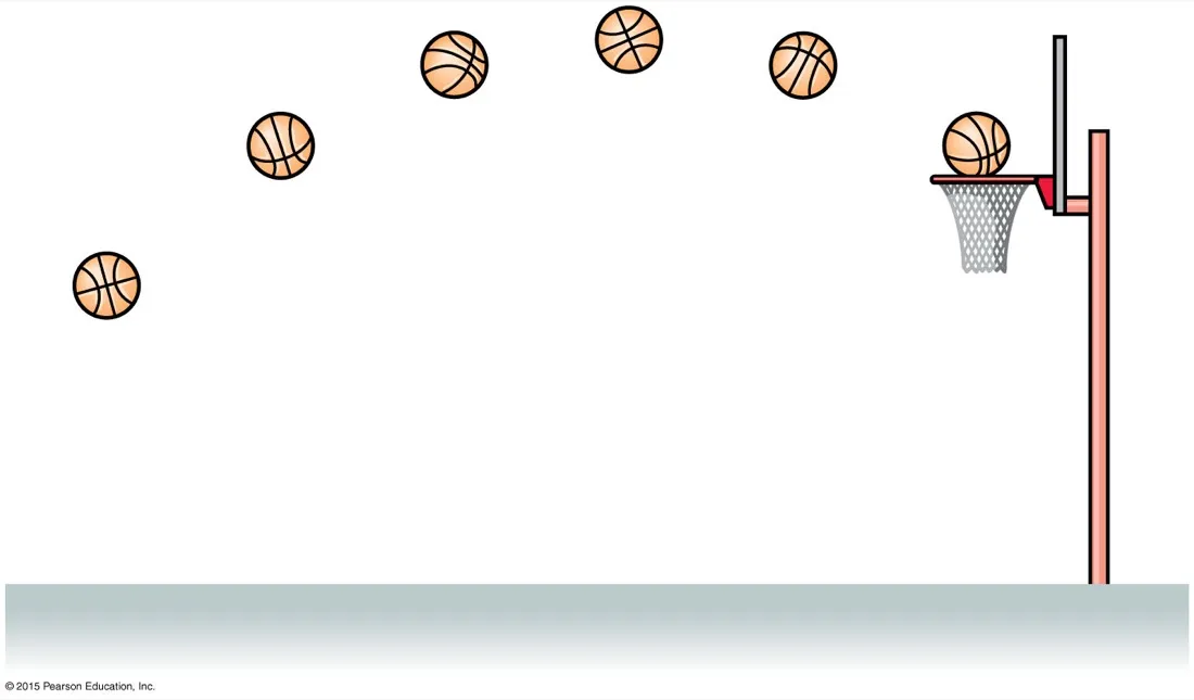
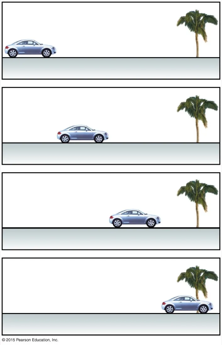
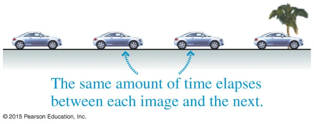
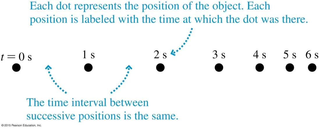
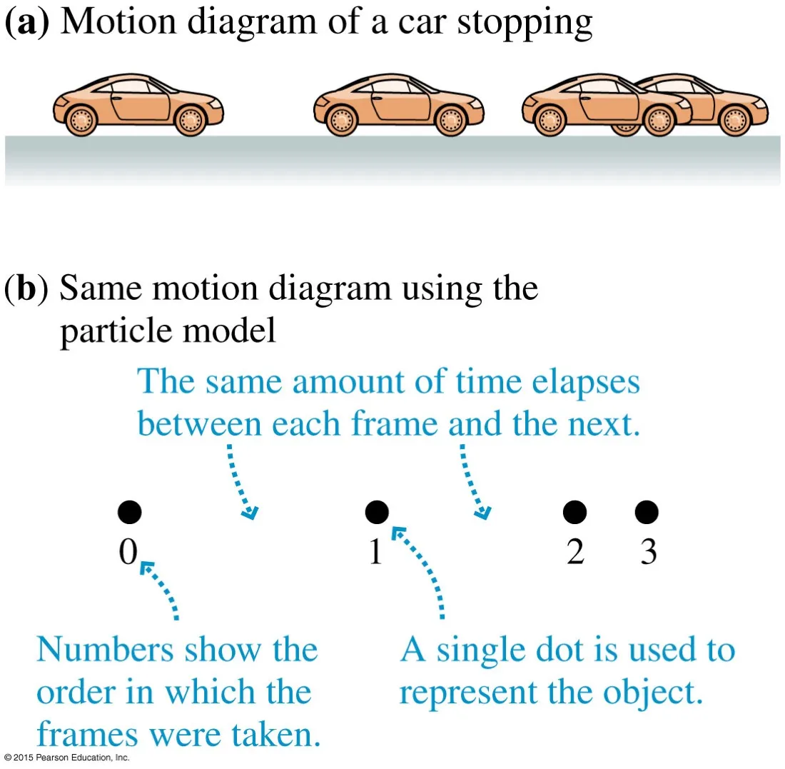
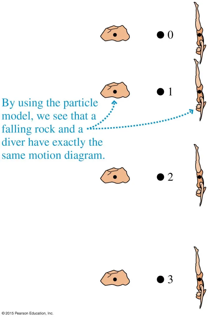
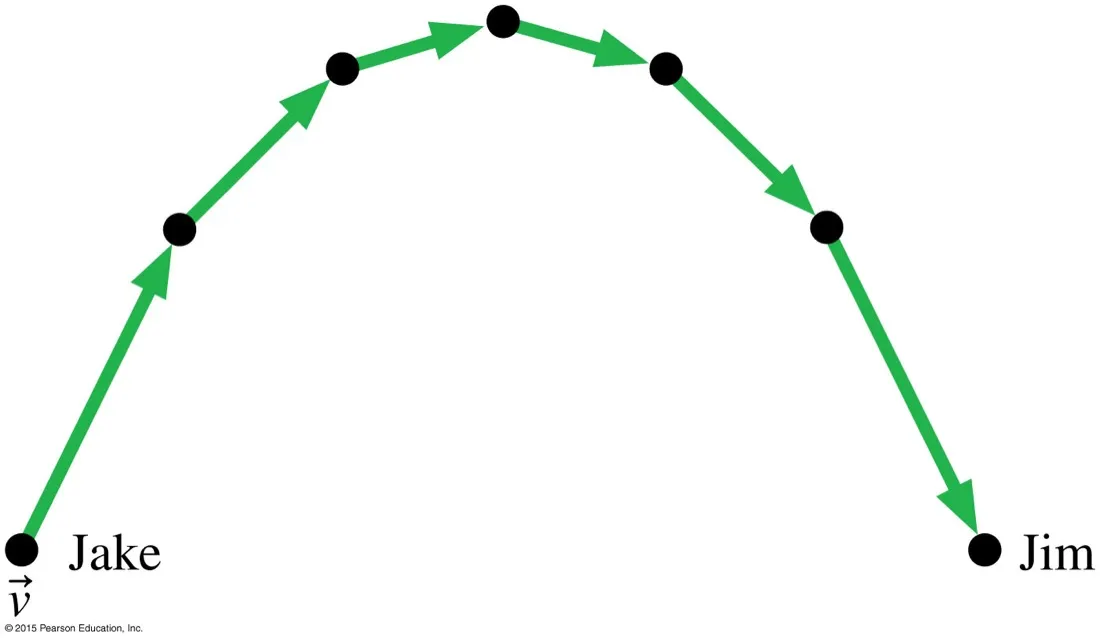
Four kinds of motionStraight-line, circular, projectile, rotational. A.1 deals with the first and the third; circular motion belongs to A.2 and rotation to A.4. Naming the type of motion first tells you which tools are legal.Equal spacing means steady speedFour frames, equal time between each. The skateboarder covers the same ground every interval, so the speed is not changing. The spacing of the frames is the whole message.Widening gaps mean speeding upSame idea, opposite reading. The gaps grow, so each equal slice of time buys more distance than the last. That is acceleration, seen before you have written a single symbol.Bunching gaps mean slowing downThe frames crowd together, so the car covers less ground per interval. Note that the car is still moving to the right the whole time — slowing down is not the same as reversing.Two-dimensional motion, same methodThe arc is a motion diagram too. Notice the horizontal spacing stays even while the vertical spacing changes — the first hint that the two directions can be treated separately.A motion diagram is just stacked framesTake a video, keep every frame, lay them out. Nothing has been idealised yet. This is the raw observation that everything else compresses.Equal time is the rule that makes it workThe frames must be equally spaced in time. If they are not, the spacing on the page tells you nothing about speed. Every motion diagram assumes this silently.Label the dots with timeEach dot is where the object was; the label is when it was there. Getting into the habit of writing the times on saves you later when you need Δt for a calculation.The particle modelReplace the object with a single dot at its centre. You lose the shape and keep the motion. This is a deliberate simplification, and knowing what you threw away is part of using it honestly.Why the particle model earns its keepA rock and a diver look nothing alike, but as particles they fall identically. This is the point: one diagram now solves both problems, and a whole class of problems you have not met yet.
A dot on a page is not yet a measurement. To get numbers you have to impose a coordinate system — and that choice is yours to make.
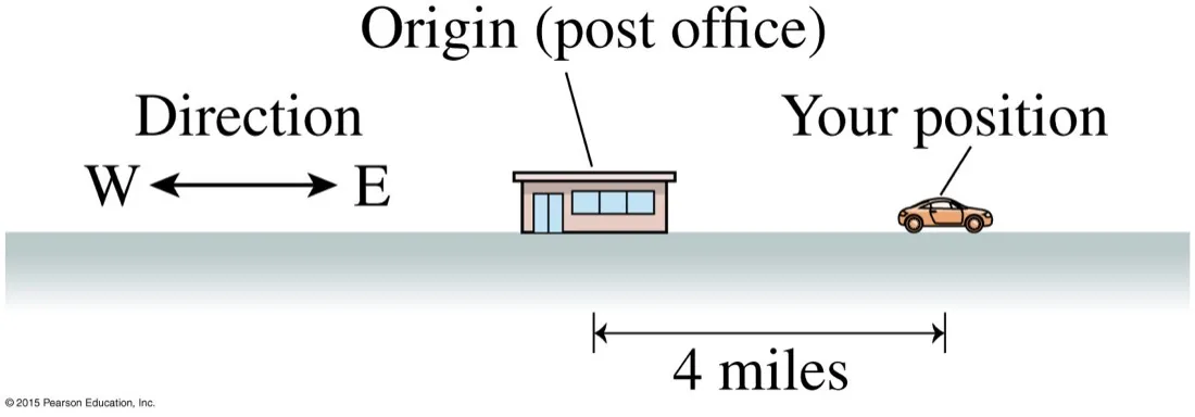
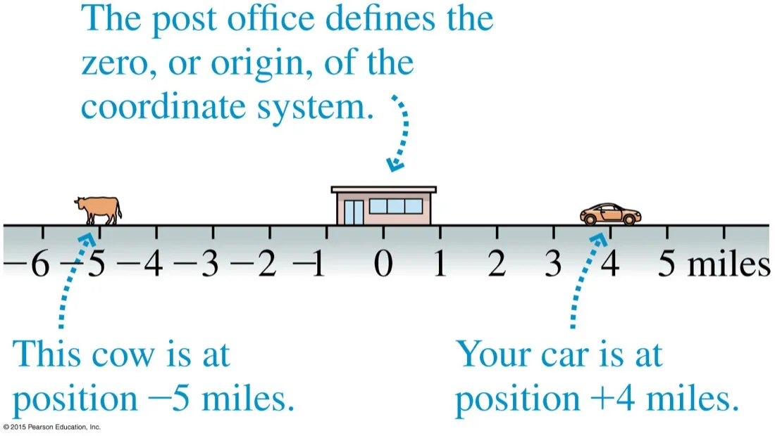
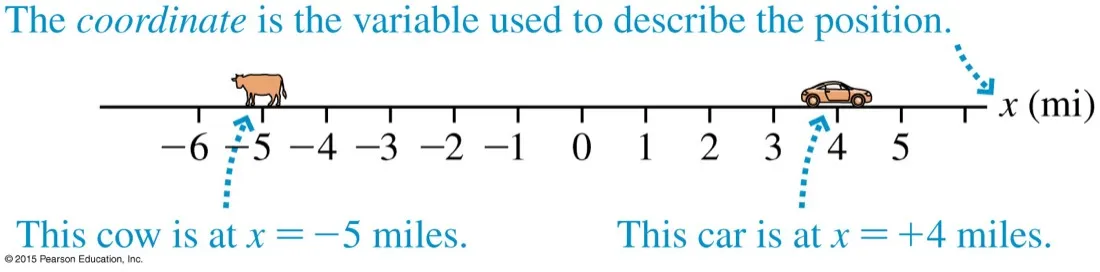
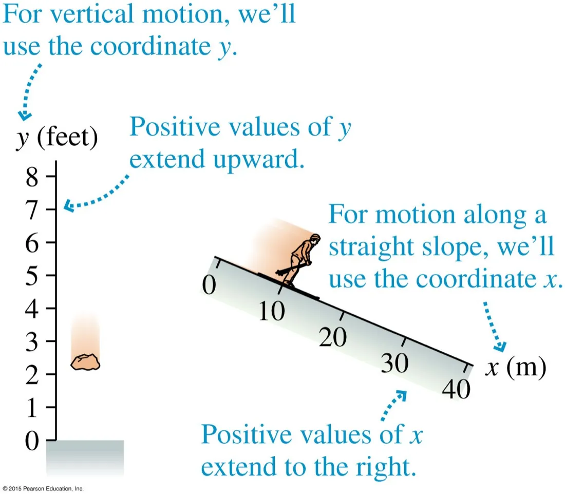
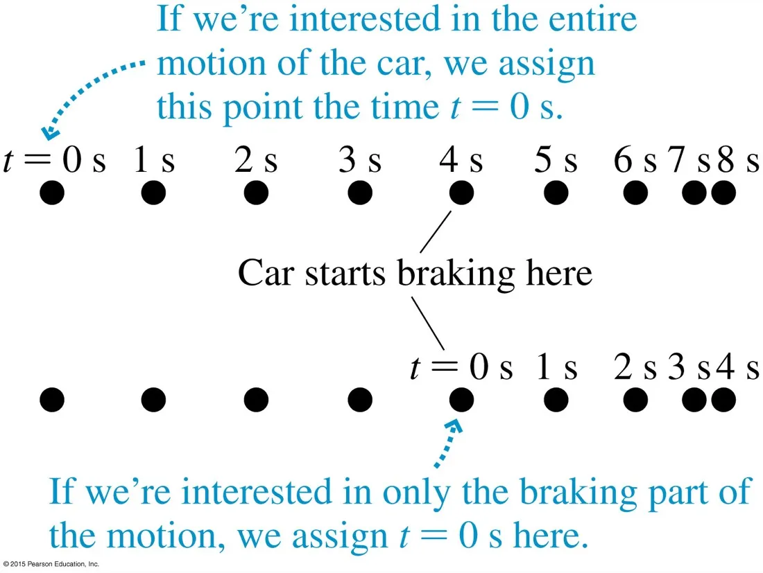
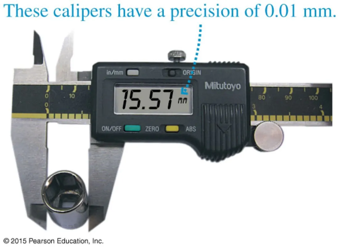
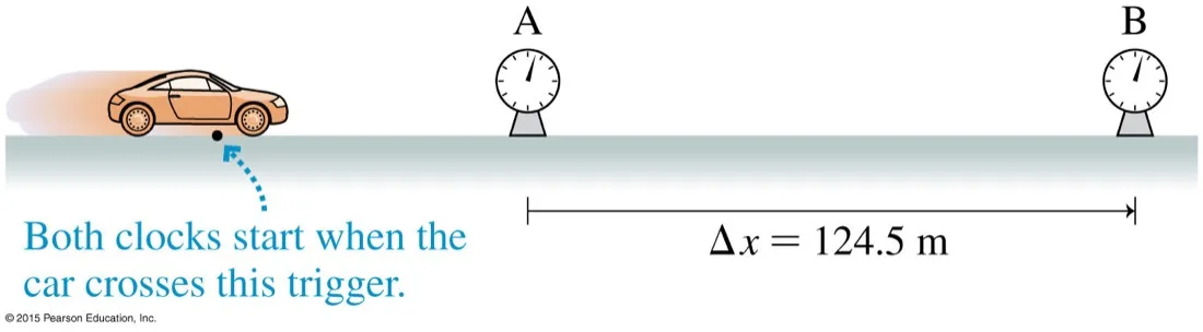
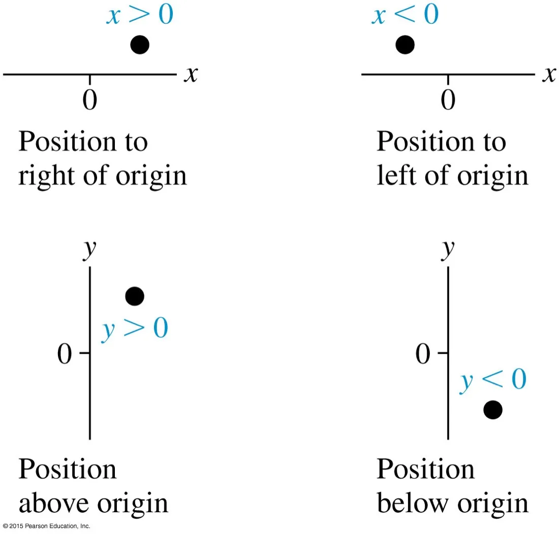
You choose the origin"Four miles from the post office" only means something once someone declares the post office to be zero. The origin is a decision, not a fact about the world.The sign carries the directionOnce the axis points east, west becomes negative. The cow is not at "5 miles the other way" — it is at −5 miles. In one dimension the sign is the entire direction information.Coordinate, not distancex is the coordinate — a signed number naming a point on the axis. It is not "how far away" anything is. Keep the two ideas apart and negative answers stop feeling wrong.Label the axis properlySymbol, then units in brackets: x (m). Choosing the start line as the origin is not required, just convenient. An unlabelled axis is the most common way to lose marks on a graph question.Pick the axis to suit the motionUse y for vertical motion, x for motion along a straight slope. The axis does not have to be horizontal — it has to lie along the motion, which makes the problem one-dimensional.Read the crowdingDots 4 and 5 nearly overlap. In equal time the object has barely moved, so it is almost at rest. You can read a stopping motion off the spacing alone.You choose t = 0 as wellBoth rows describe the identical car. If you only care about the braking, start the clock there and the numbers get smaller. Moving the origin of time is free and often makes the algebra easier.Precision is a property of the instrumentThese calipers resolve to 0.01 mm, so 15.57 mm is honest and 15.5700 mm is a lie. The instrument sets how many figures you are entitled to write down.Measuring, not assumingΔx is measured to four figures here, but the clocks will be the weak link. When you divide these to get a speed, the answer inherits the worse of the two precisions.
The single most examined distinction in A.1, and the one students most often get wrong under pressure.
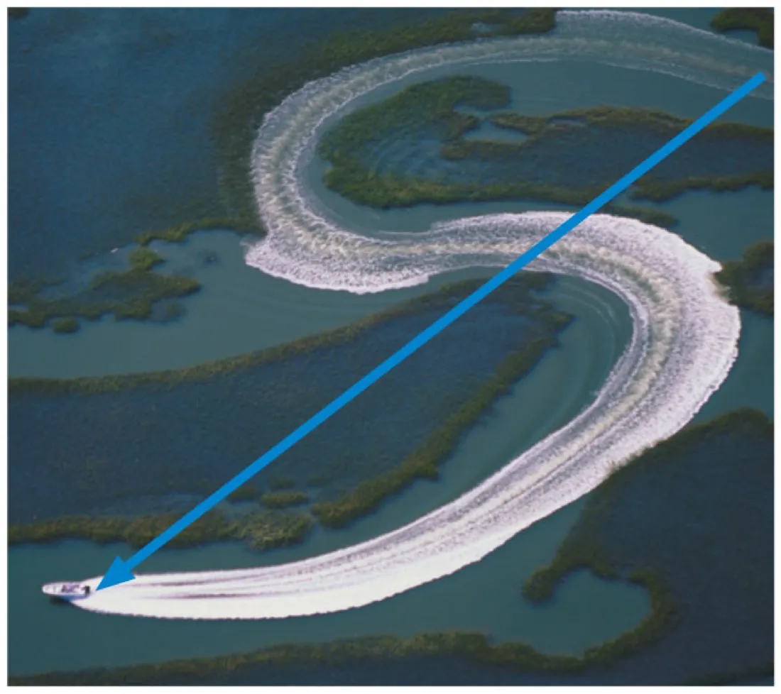
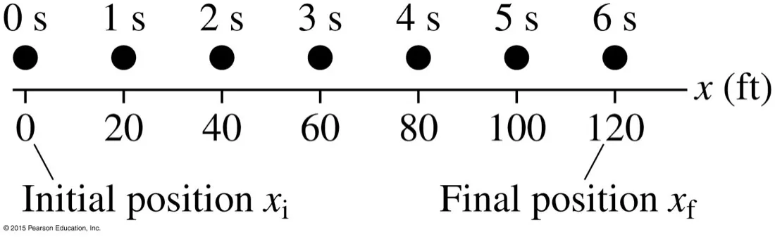
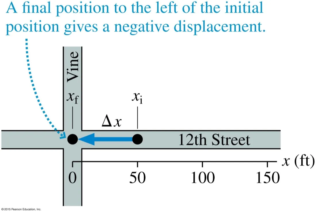
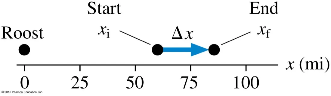
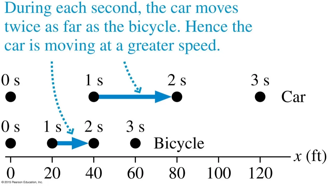
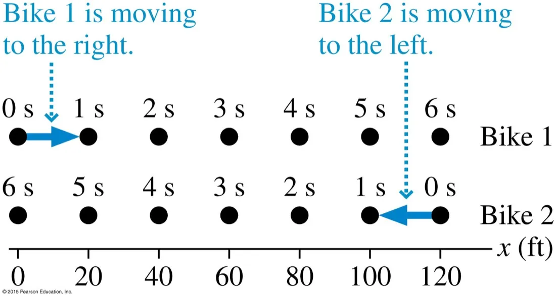
Distance is the wake; displacement is the arrowThe boat travelled every metre of that curling wake. Its displacement is the straight arrow — start to finish, nothing else. If it had looped back to where it began, the displacement would be zero and the distance enormous.Δx = xf − xiFinal minus initial, always in that order. Here 120 − 0 = +120 ft. Writing it the other way round is the single commonest sign error in the topic.Negative displacement0 − 50 = −50 ft. The minus sign is not an error to be tidied away; it is the answer telling you the motion was westward. Distance travelled here is still +50 ft.Displacement does not care about the originThe roost sits at zero but the journey starts at 60. Δx is the same whatever you called the origin — shift the axis and both positions shift together. Position depends on the origin; displacement does not.Comparing speeds from spacingSame clock, double the spacing, double the speed. You can rank speeds off two motion diagrams without computing anything, provided the time between frames is the same for both.Read the time labels, not the layoutBoth rows look identical until you read the numbers. Bike 2's clock runs right to left, so it is travelling in the negative direction. Always check which way time increases before you call a sign.Speed is relative to somethingThe rider is frozen and the world is smeared, because the camera moved with the bike. In the bike's frame the trees are the ones moving. Every velocity is quoted relative to a chosen frame, usually the ground.
In one dimension a sign is enough. The moment motion leaves the line you need vectors, and the trig that goes with them.
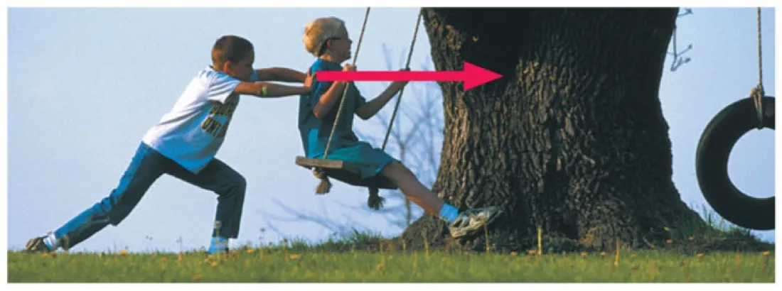
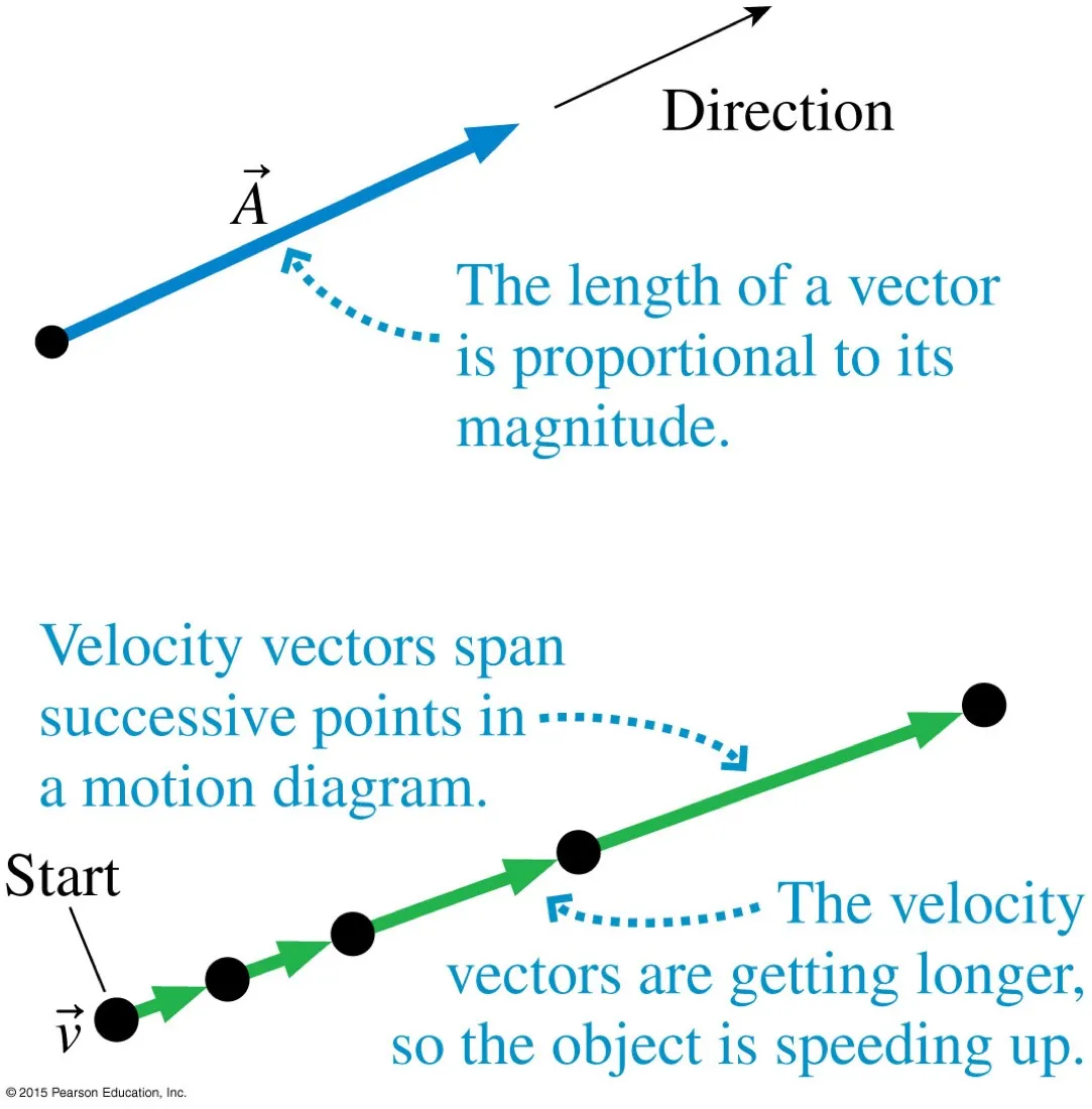
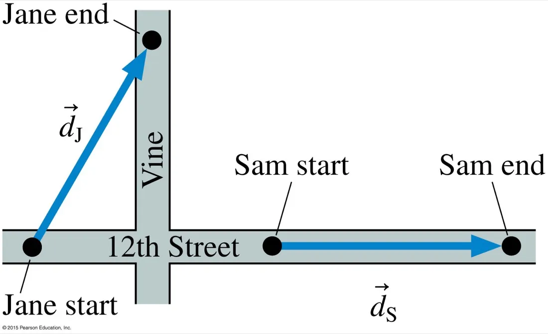
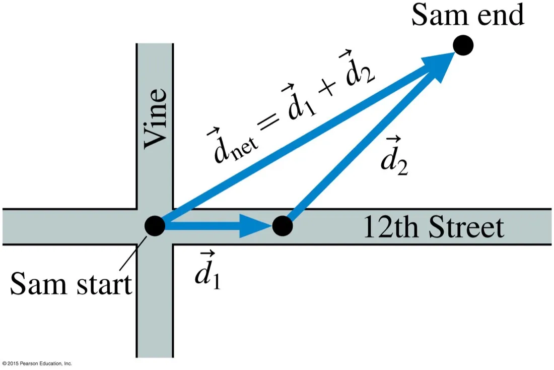
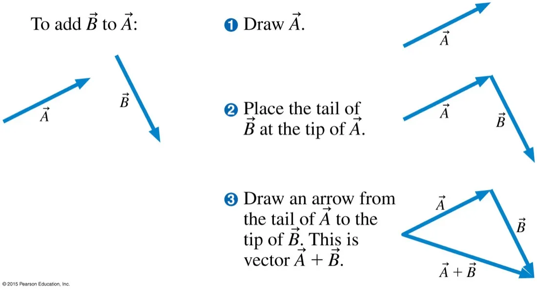
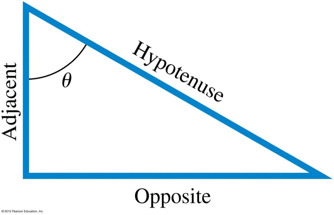
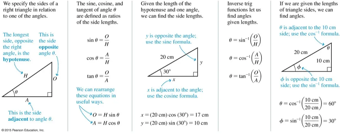
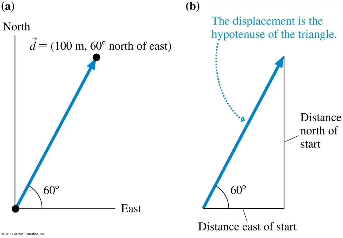
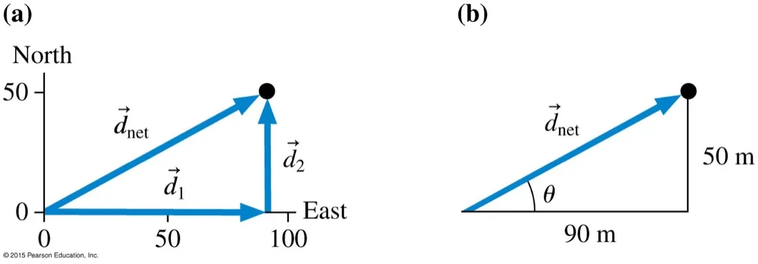
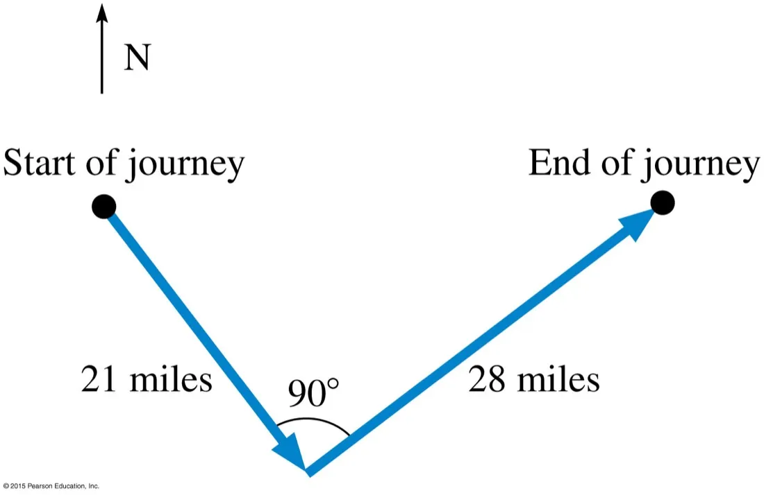
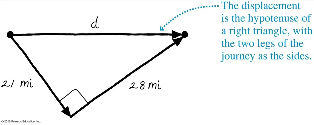
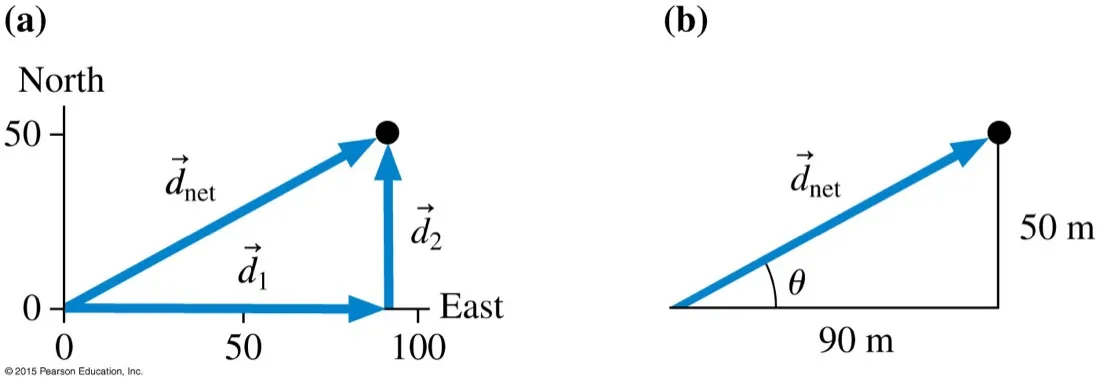
A vector has size and directionThe arrow says how hard and which way. Change either and you have a different vector. A scalar — mass, time, distance — has no arrow to draw.Length on the page means magnitudeDraw vectors to scale and the diagram does arithmetic for you. Velocity vectors span successive dots; if they lengthen, the object is speeding up. Sloppy arrow lengths throw that away.Same streets, different displacementsJane and Sam both walked; their displacement vectors differ in both length and direction. Two vectors are equal only when magnitude and direction match — position on the page is irrelevant.Adding vectors tip to tailWalk one leg, then the next; the net displacement is the single arrow from where you started to where you stopped. It is shorter than the distance you actually walked — that is the whole point.The method, in three stepsDraw A. Put B's tail on A's tip. Draw from A's tail to B's tip. Do it in this order every time and the geometry never confuses you, however many vectors you are chaining.Naming the sidesOpposite and adjacent are defined relative to the angle you picked, not to the page. Move θ to the other acute angle and the two labels swap. Fix θ first, then name.Everything trigonometric you need for A.1Sides from an angle: multiply by sin or cos. Angle from sides: use the inverse. There is nothing beyond this panel in the whole of A.1 — worth keeping open until it is automatic.Every vector hides a right triangleDrop a perpendicular and the vector becomes the hypotenuse. The legs are the components: 100 cos 60° east, 100 sin 60° north. This move is what makes two-dimensional problems solvable.And back againGiven the legs, Pythagoras gives the magnitude and tan⁻¹(50/90) gives the angle. Going vector → components → vector is the round trip you will make constantly from A.2 onwards.Set the problem up firstTwo legs at 90°. Before reaching for a calculator, notice the right angle — it is what makes this solvable with Pythagoras rather than the cosine rule.The sketch is the workingRedrawn by hand, deliberately rough. A sketch this crude is enough to see that d = √(21² + 28²) = 35 miles. Draw before you calculate, every time.
Unglamorous, heavily penalised in exams, and the subject of one of the most expensive mistakes in spaceflight history.
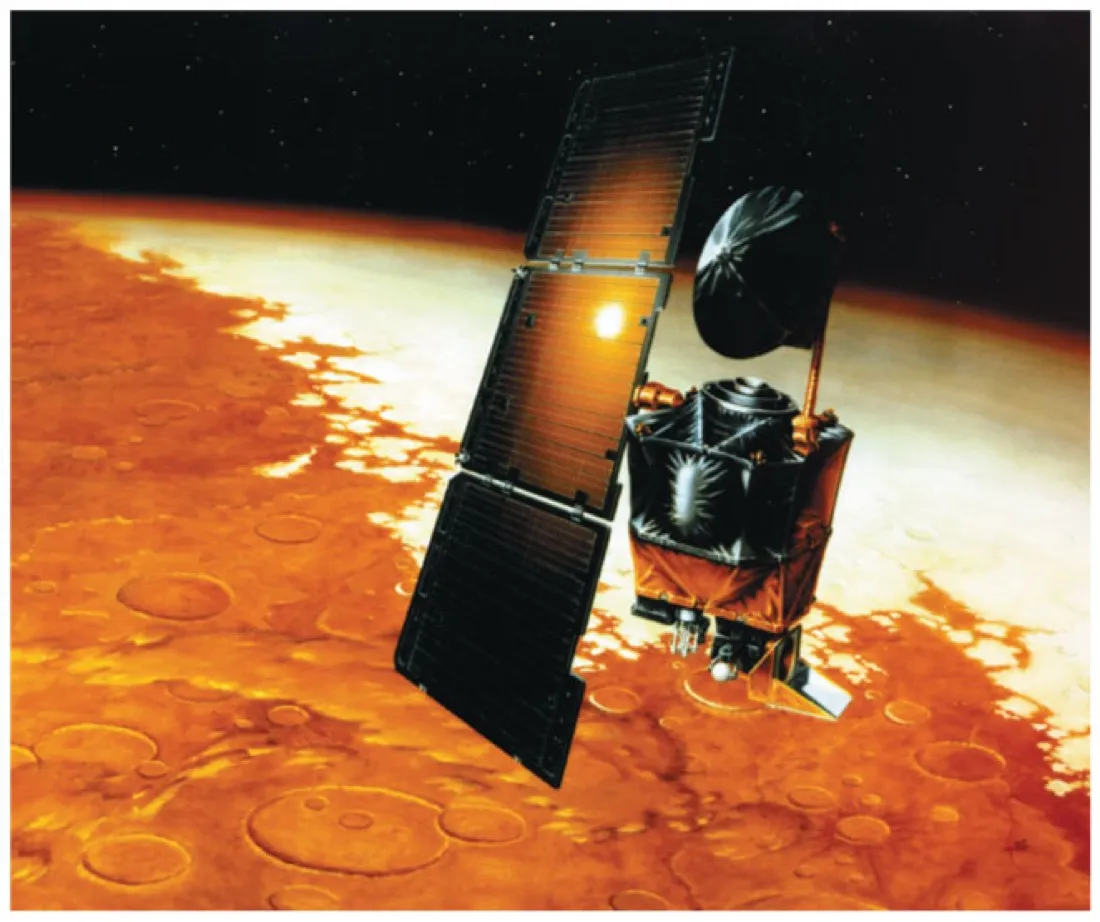
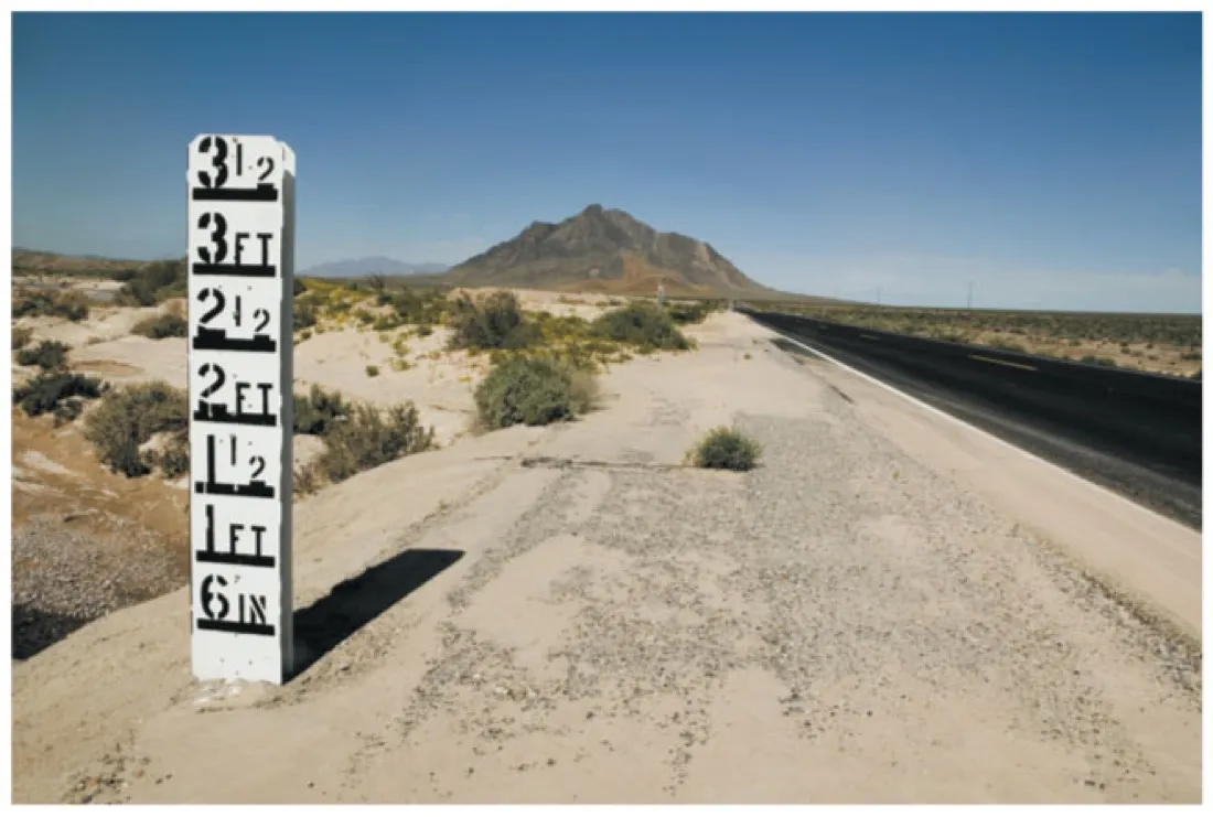
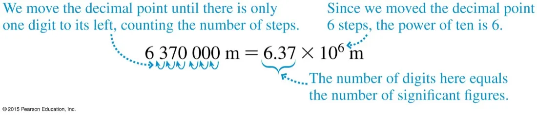
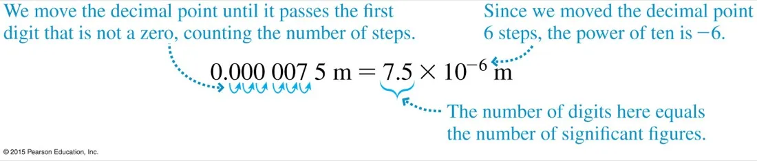
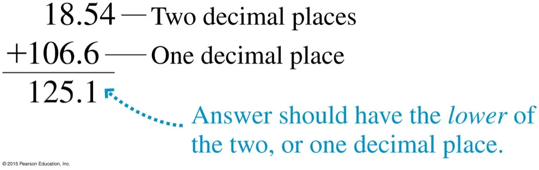
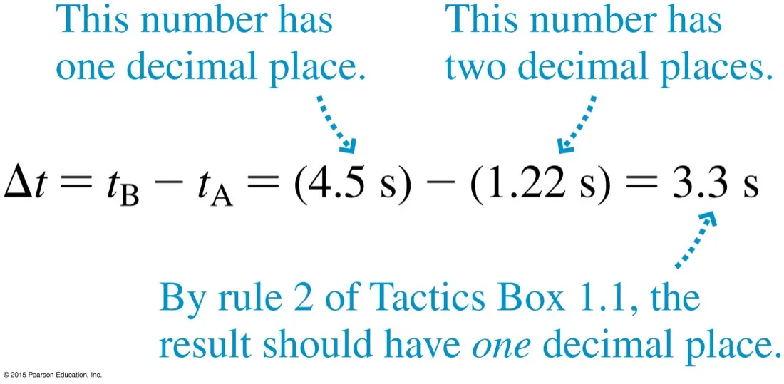
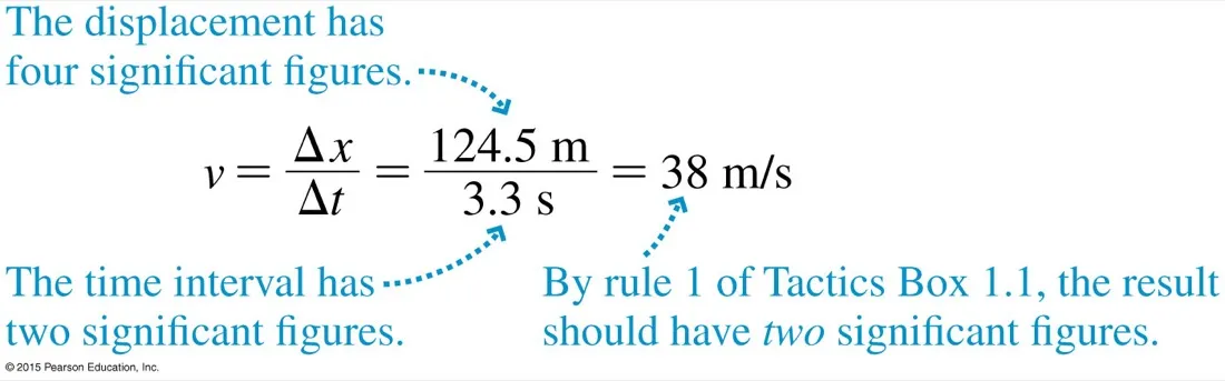
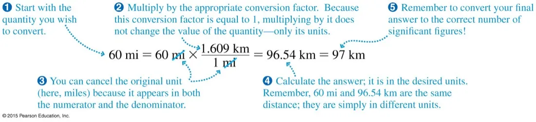
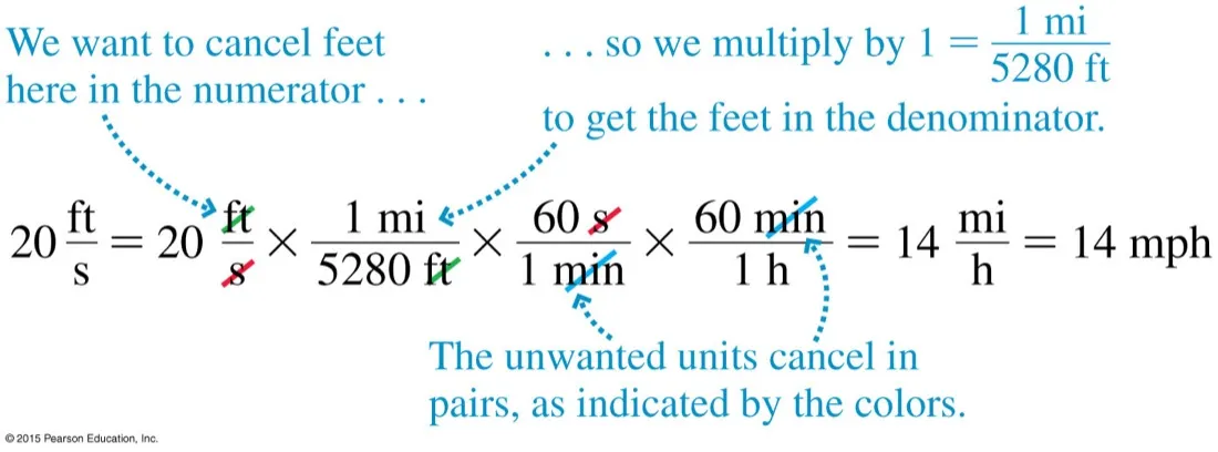
What units costThe Mars Climate Orbiter was lost in 1999 because one team worked in pound-seconds and another in newton-seconds. £100 million, destroyed by an unstated unit. Write the units down.Scales are chosen for a purposeMarked in feet and inches because that is what the people reading it use. Physics standardises on SI so that nobody has to guess — but the world it measures rarely does.Scientific notation, large numbersMove the point until one digit sits to its left; count the steps for the exponent. The form also settles the ambiguity — 6.37 × 10⁶ is unmistakably three significant figures.Scientific notation, small numbersSame rule, negative exponent. The leading zeros are placeholders and never count as significant — here there are two significant figures, not eight.Multiplying: fewest significant figures winsThree figures times two figures gives two. The calculator says 21.261; you write 21. Extra digits are not extra accuracy, they are a claim you cannot support.Adding: fewest decimal places winsA different rule from multiplication, and the reason marks get lost. Adding and subtracting go by decimal places; multiplying and dividing go by significant figures.The rule in action — subtraction4.5 has one decimal place, so the answer gets one: 3.3 s, not 3.28 s. The coarser measurement sets the limit, and here it throws away a digit before you have even started.The rule in action — divisionA displacement good to four figures divided by a time good to two gives a velocity good to two: 38 m s⁻¹. Careful distance measurement is wasted if the timing is sloppy — worth remembering in the lab.Conversion factors are just multiplying by one1.609 km / 1 mi equals 1, so multiplying by it changes the units and not the quantity. Cancel the unwanted unit on the page and you cannot get the conversion upside down.Chaining conversionsThree factors in a row, each cancelling one unwanted unit. Chain them in a single line rather than converting in stages — fewer intermediate roundings and much easier to check.
Motion diagrams get unwieldy fast. The graph is where kinematics starts to become quantitative.
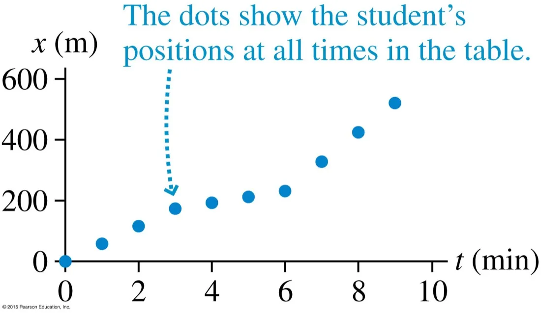
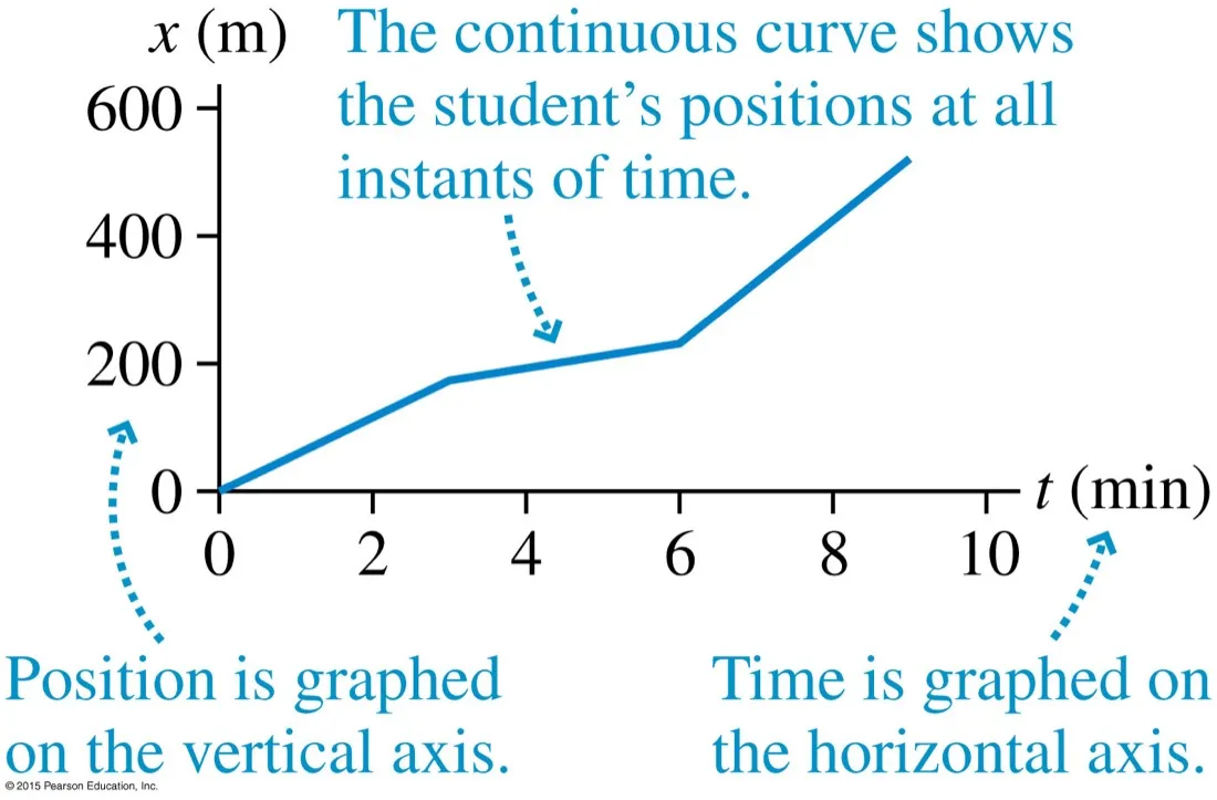
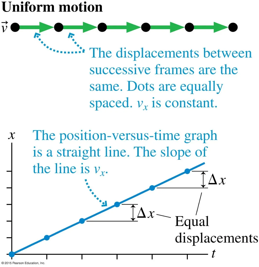
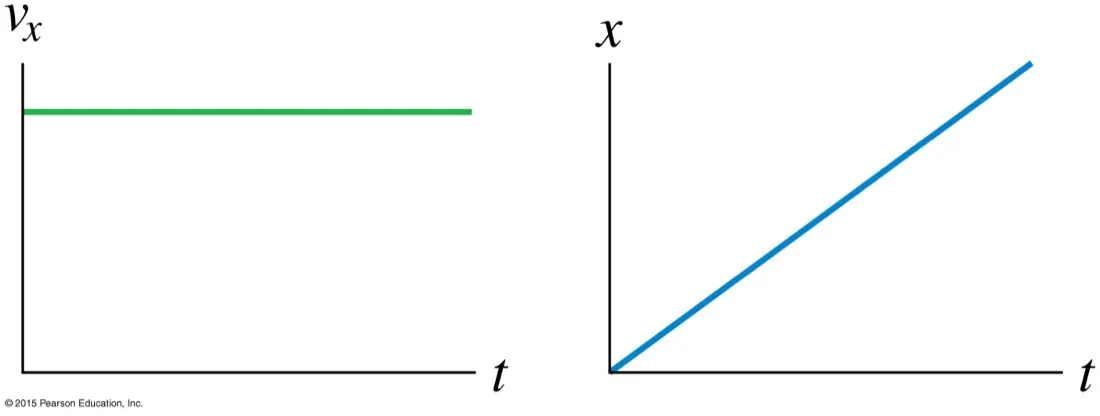
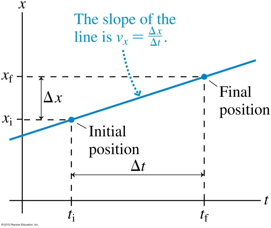
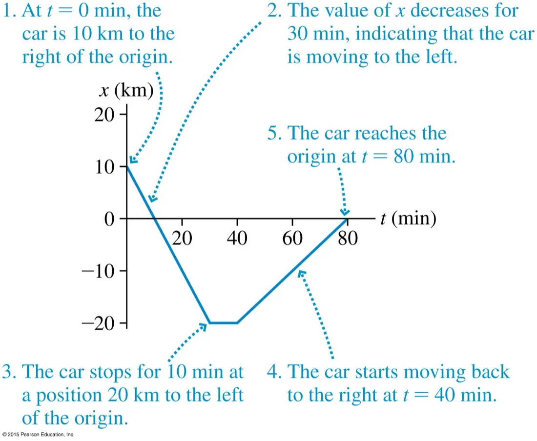
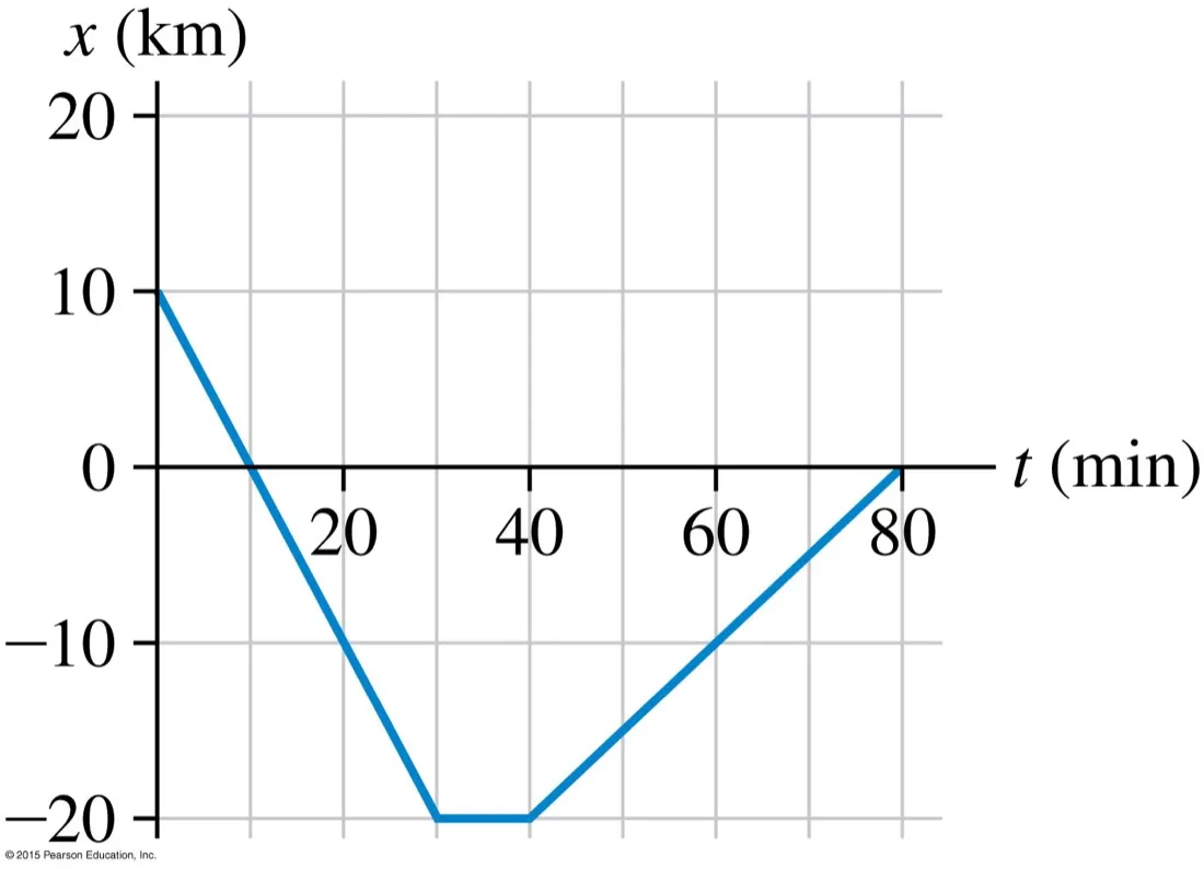
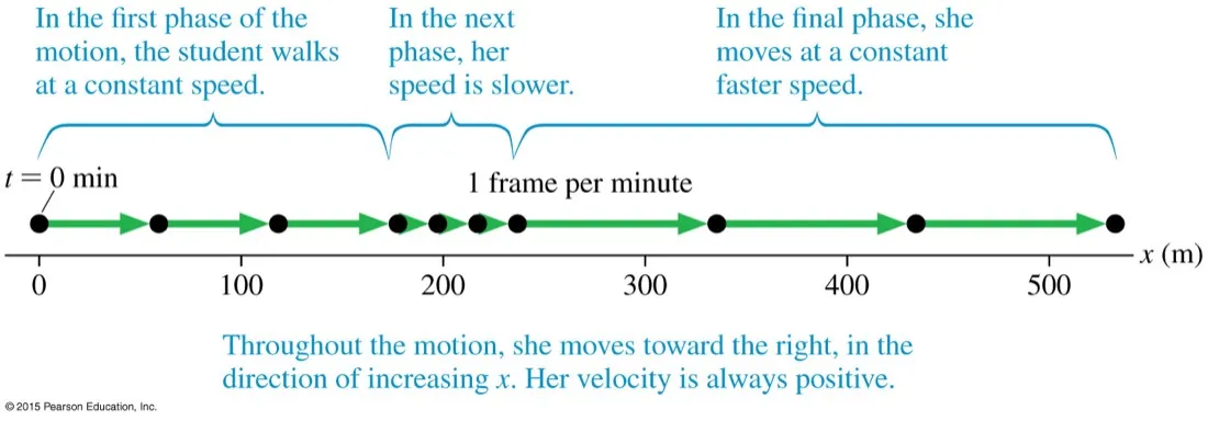
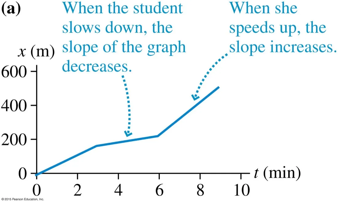
The sign convention, fixed onceRight and up are positive by default. You may choose otherwise, but choose before you start and never mid-problem. Most sign errors are really convention changes made halfway through.A real journey as dotsOne frame per minute over about nine minutes. The crowding near 200 m says she slowed there. Getting a number out of this by counting dots is possible but painful — hence the graph.The same walk, plottedEach dot is one row of the table: a time and the position at that time. Nothing has been added yet — this is the motion diagram with time given its own axis.Joining the dots is a claimThe line asserts she had a position at every instant between measurements, which is reasonable for a walking student. Position on the vertical axis, time on the horizontal — always this way round.Uniform motion is a straight lineEqual displacements in equal times, so the graph is straight and the slope constant. "Uniform" means constant velocity, which means zero acceleration — not merely "moving".The shape pair to memoriseFlat v–t goes with straight x–t. Learn these as a pair; a huge number of multiple-choice questions are testing exactly this correspondence and nothing else.Slope is velocityRise over run, with units. Δx in metres over Δt in seconds gives m s⁻¹ automatically — which is a useful check that you have read the axes the right way round.Reading a graph as a storyFive features, five sentences. Downward slope means moving in the negative direction; flat means stopped; the crossing at 80 min is the return to the origin. Practise narrating graphs before calculating from them.Now without the annotationsThe same journey stripped of help. Cover the previous figure and narrate this one yourself — where is it moving fastest, where is it stationary, when does it pass the origin?
The first of the two graph relationships that carry the whole topic. Get this one solid and half of A.1 follows.
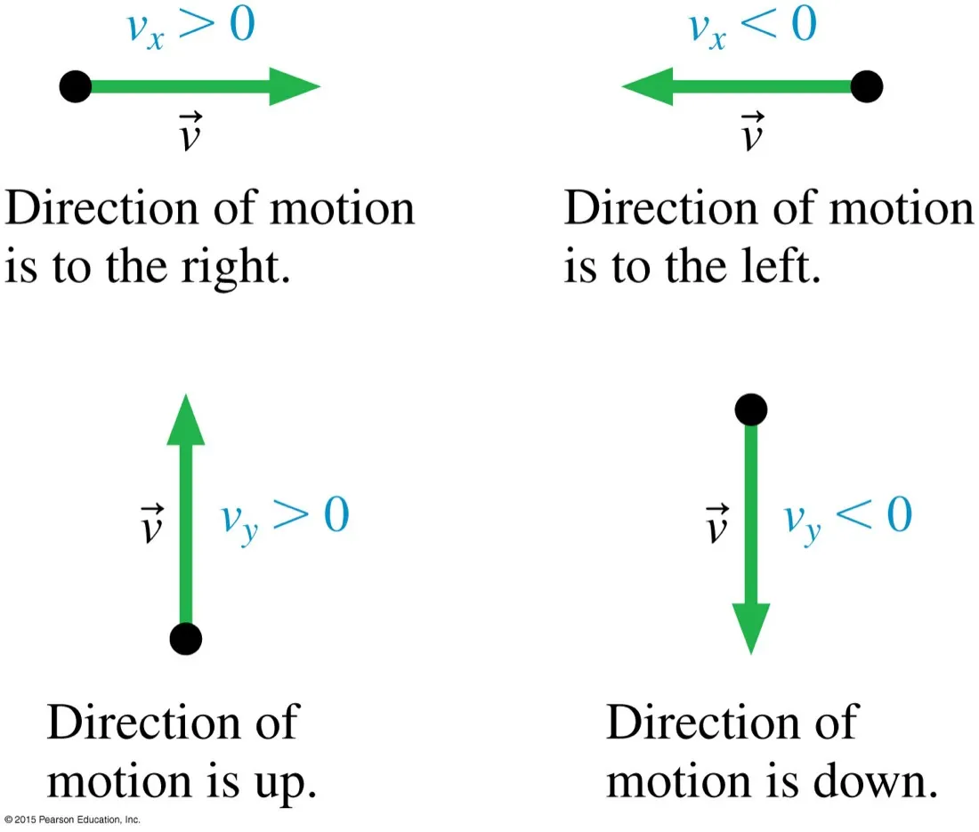
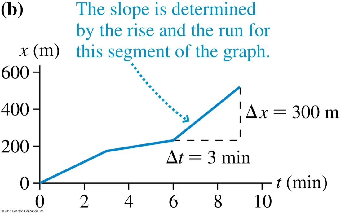
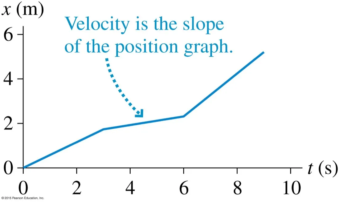
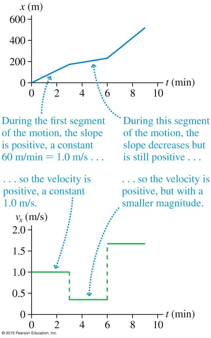
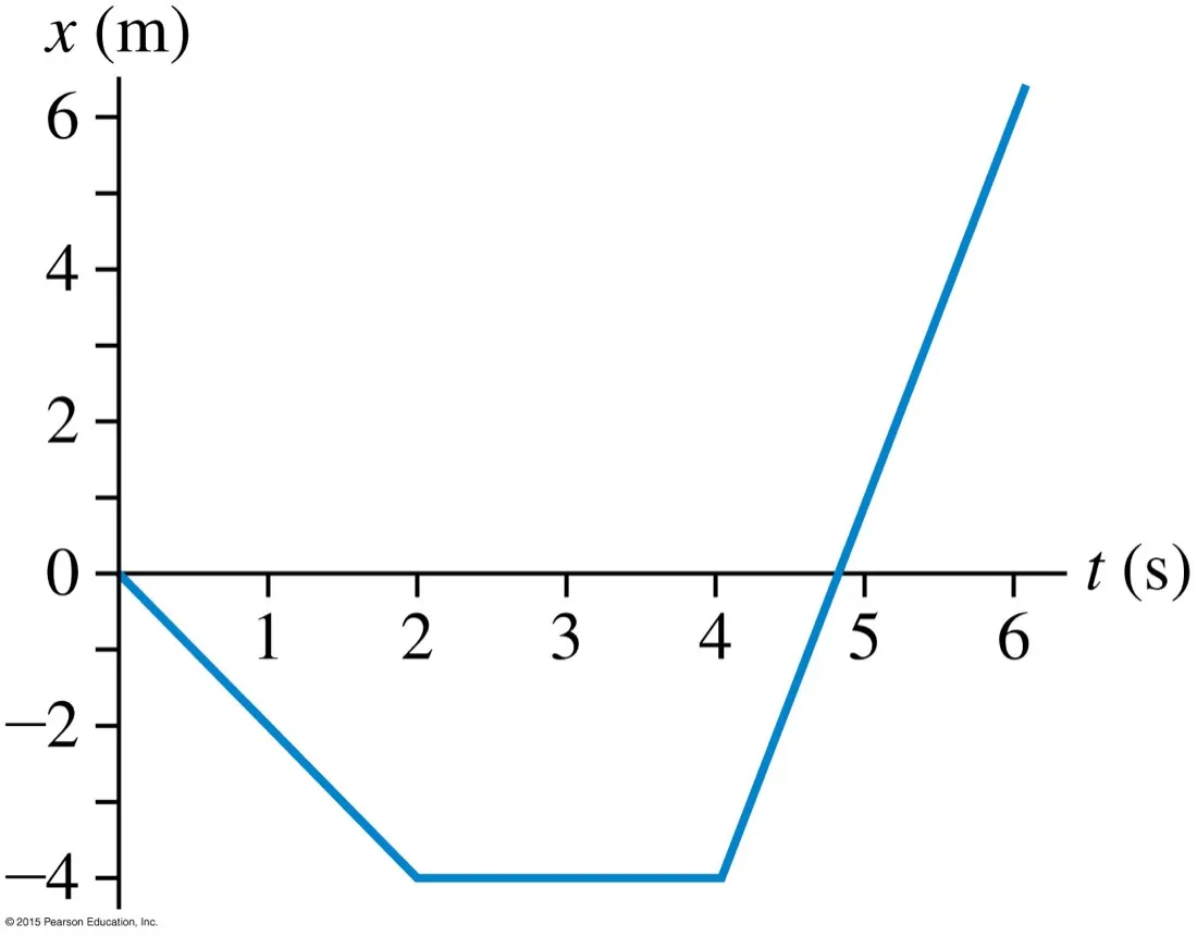
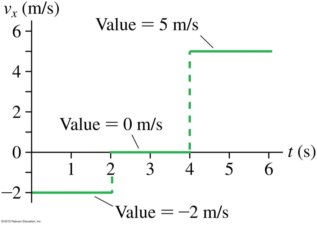
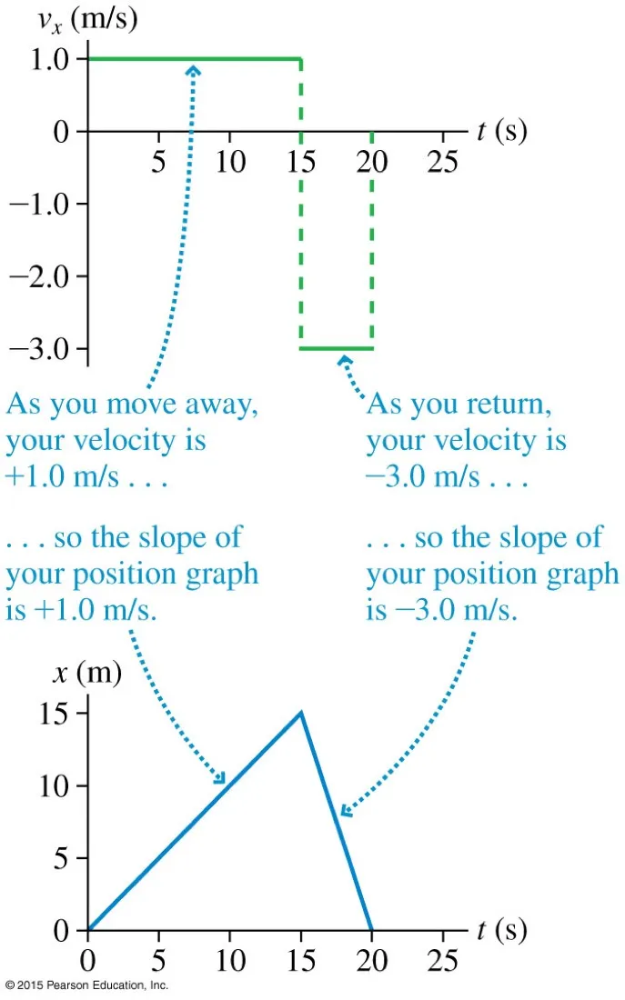
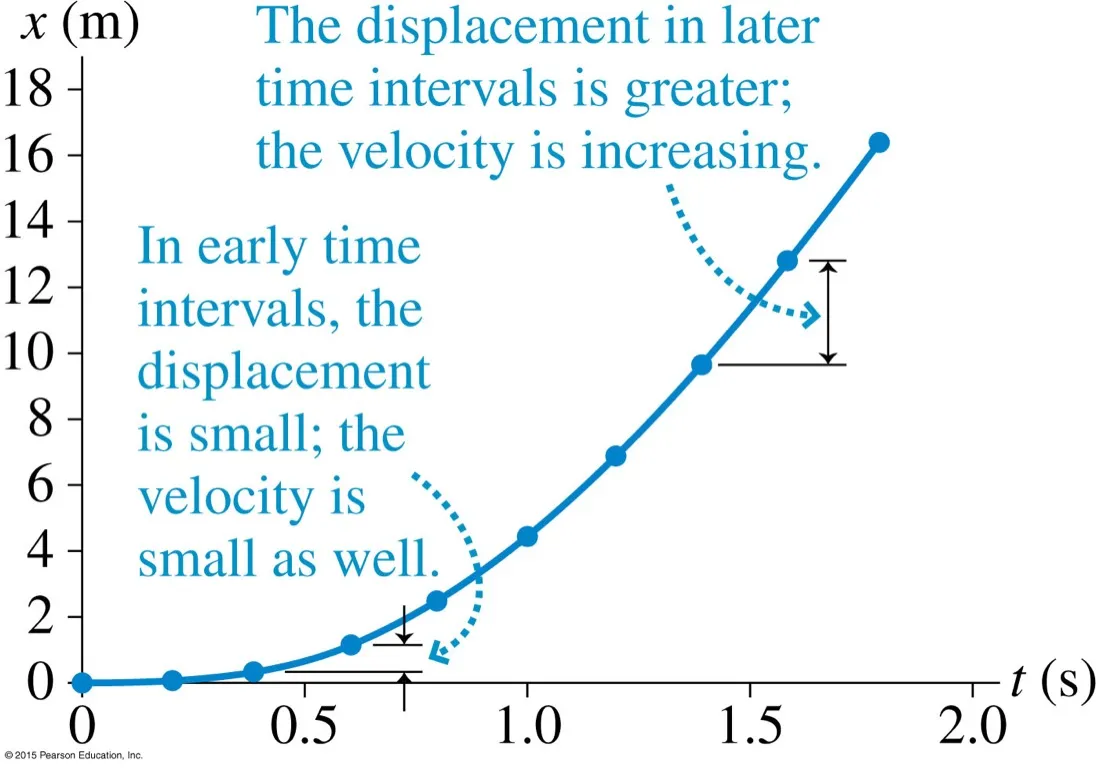
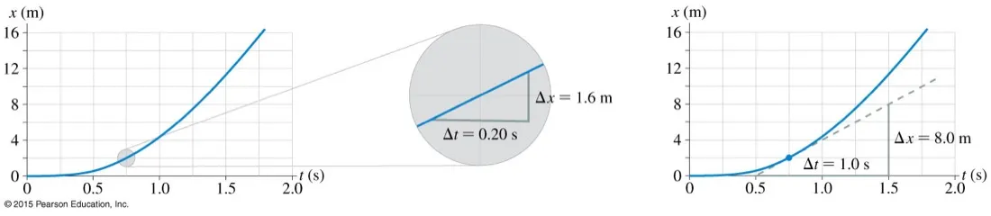
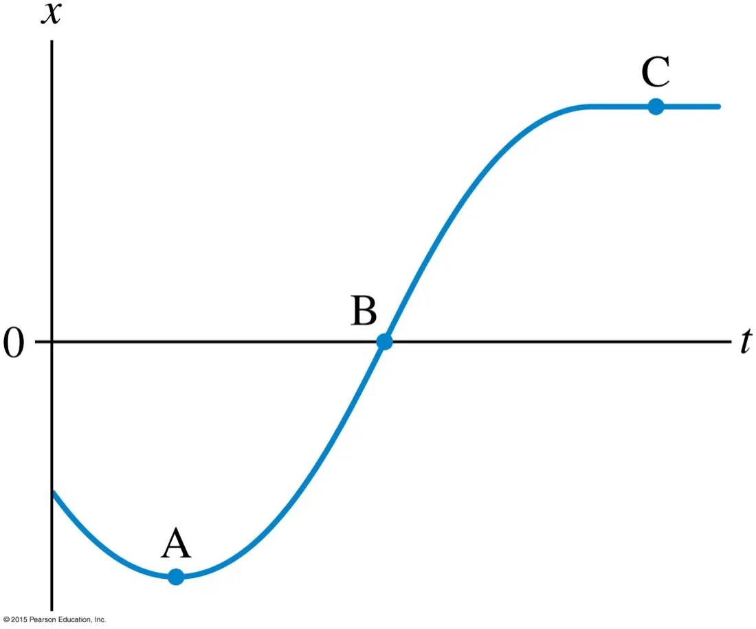
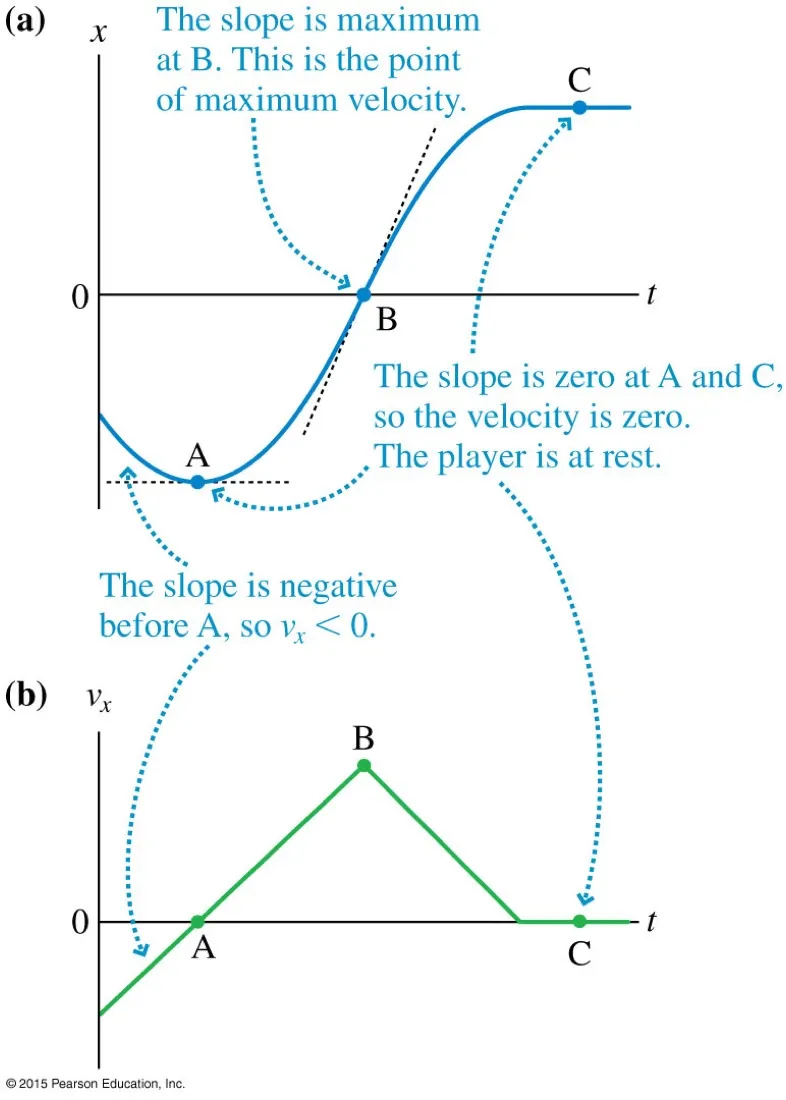
The sign of the velocity is the directionOnce the axis is chosen the sign says everything about direction. In one dimension you never need an angle — a plus or a minus does the whole job.Slower is not backwardsThree phases, three speeds, one direction. Her velocity is positive throughout even while she is slowing — a distinction the next few figures depend on completely.Slope tracks speedThe graph flattens where she dawdles and steepens where she hurries. You are reading a rate off a shape, which is the single most transferable skill in the course.Taking the numbers off300 m in 3 min. Convert before you divide: 300 m / 180 s = 1.7 m s⁻¹. Take the triangle over a large, clearly readable interval — small triangles magnify your reading errors.The statement itselfWorth writing on the inside cover of your notes. Velocity is the slope — not related to it, not proportional to it. Everything in this section is a consequence.Deriving v–t from x–tRead the slope of each straight segment above, plot it as a height below. Straight segments give flat steps. This is differentiation done by eye, and it is exactly what the exam asks for.Practise on this oneThree segments: negative slope, zero slope, steep positive slope. Sketch the velocity graph before looking at the next figure — that is the intended order.The answer−2 m s⁻¹, then 0, then +5 m s⁻¹. The vertical dashes are not real — velocity cannot jump instantly. They are an artefact of pretending the corners on the position graph were sharp.Out and backAway at 1.0 m s⁻¹, back at 3.0 m s⁻¹ — three times faster, so a third of the time. Note the return is steeper and negative, and that she ends where she began: displacement zero, distance 30 m.When the graph curvesEqual time slices, growing displacements. A curved x–t means the velocity is changing, so a single slope no longer describes the whole motion.Instantaneous velocity is the tangentShrink the interval and the curve straightens; the limit is the tangent. Both readings give 8.0 m s⁻¹ at that instant. Draw the tangent long — a short one is impossible to measure accurately.Where is it fastest?Three points, three different slopes. Decide the sign and rough size of the velocity at A, B and C before turning to the next figure.The answerZero slope at A and C means at rest — a turning point, not a stop in the story. Maximum slope at B gives peak velocity. A minimum on x–t is a zero on v–t, never a minimum.
The second graph relationship, and the one students reach for least often — usually to their cost.
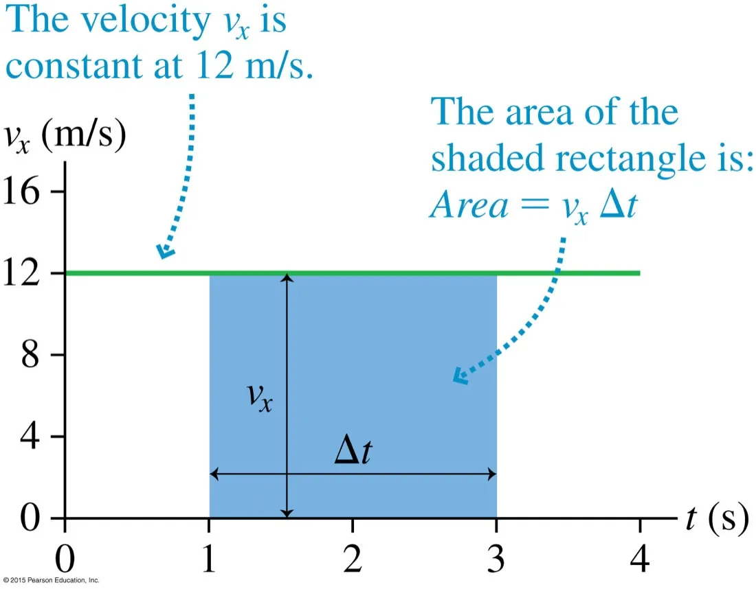
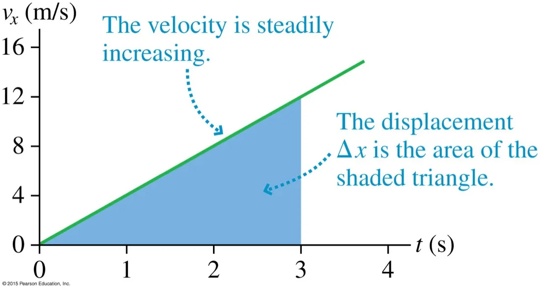
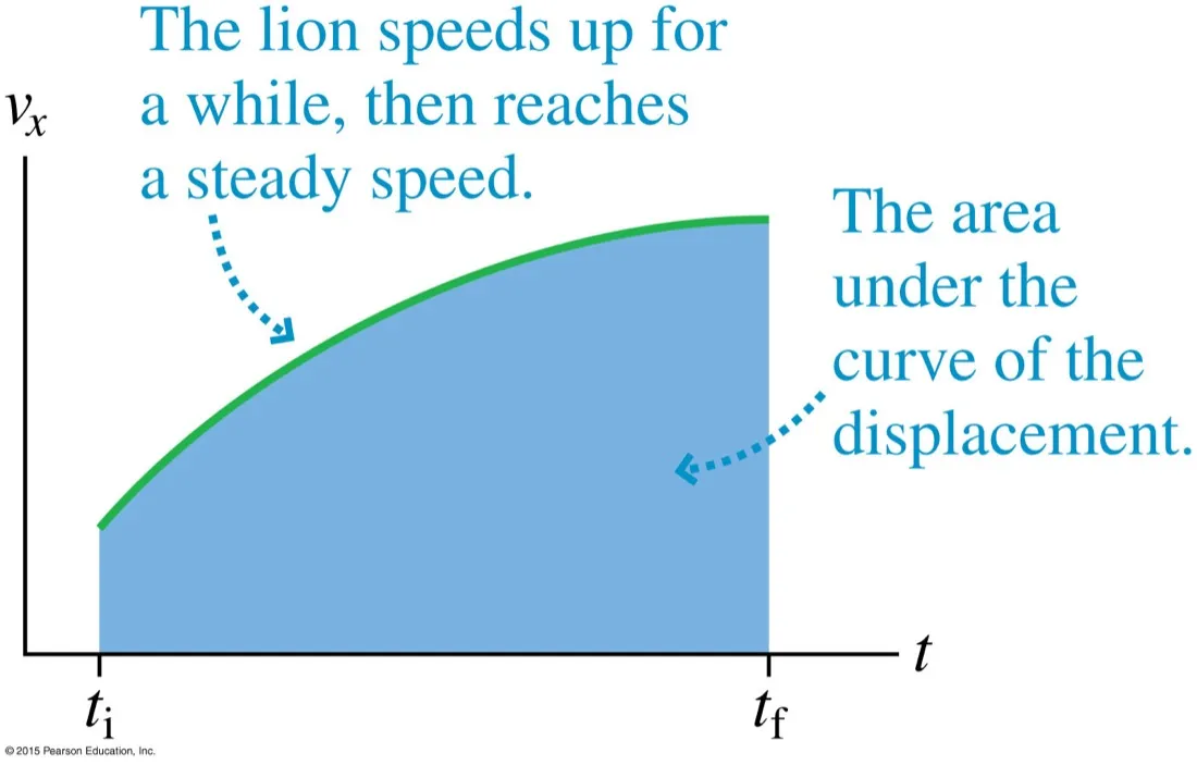
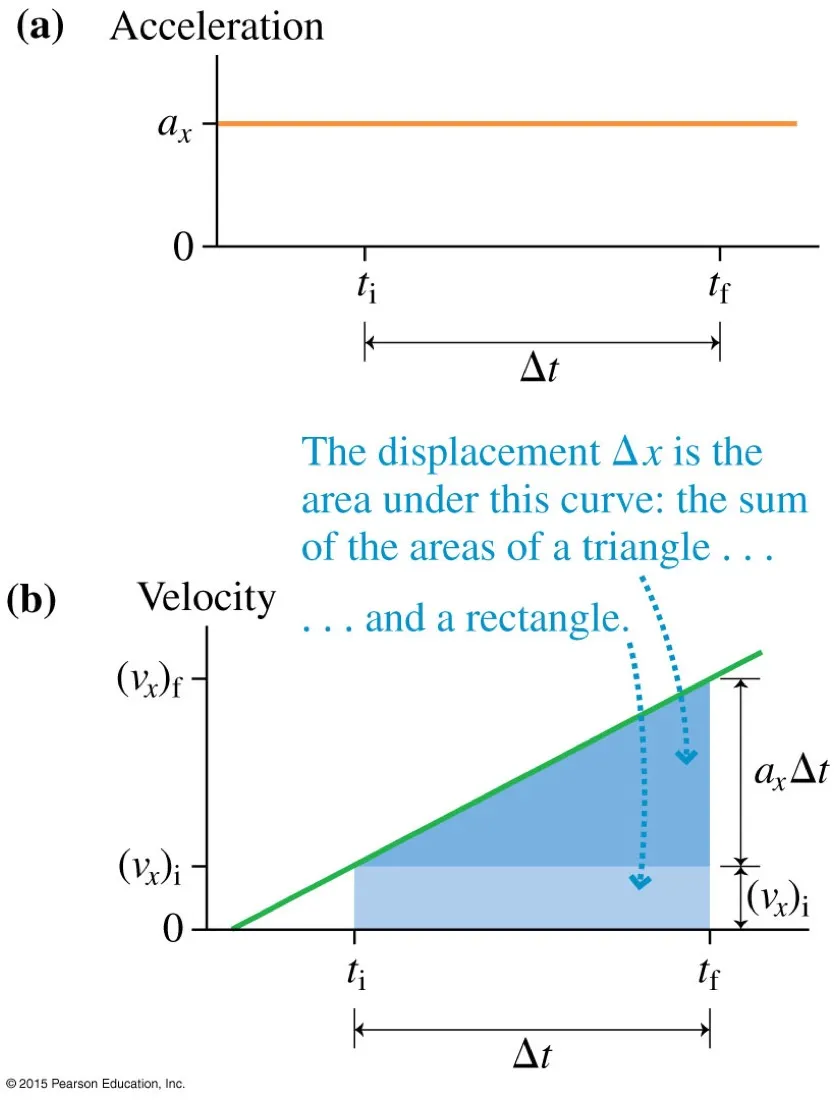
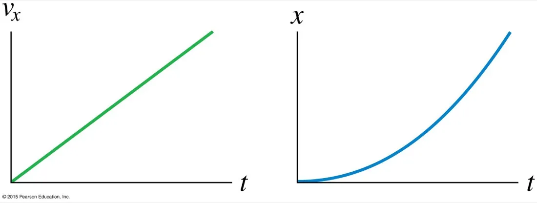
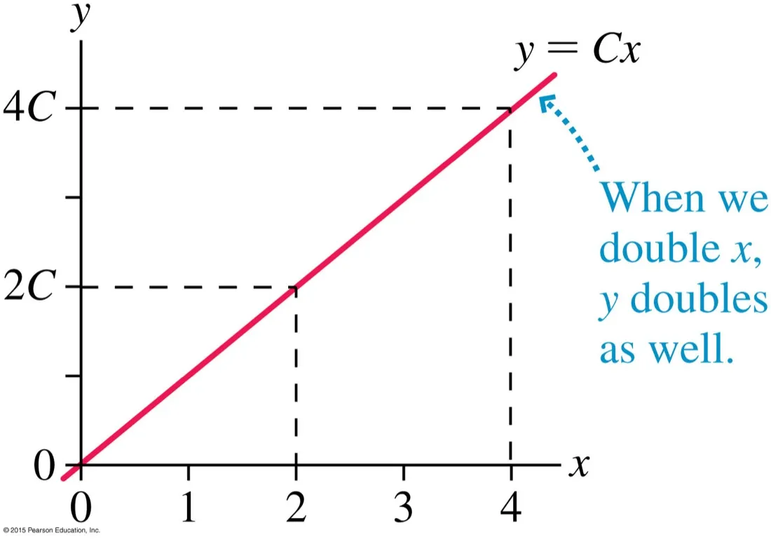
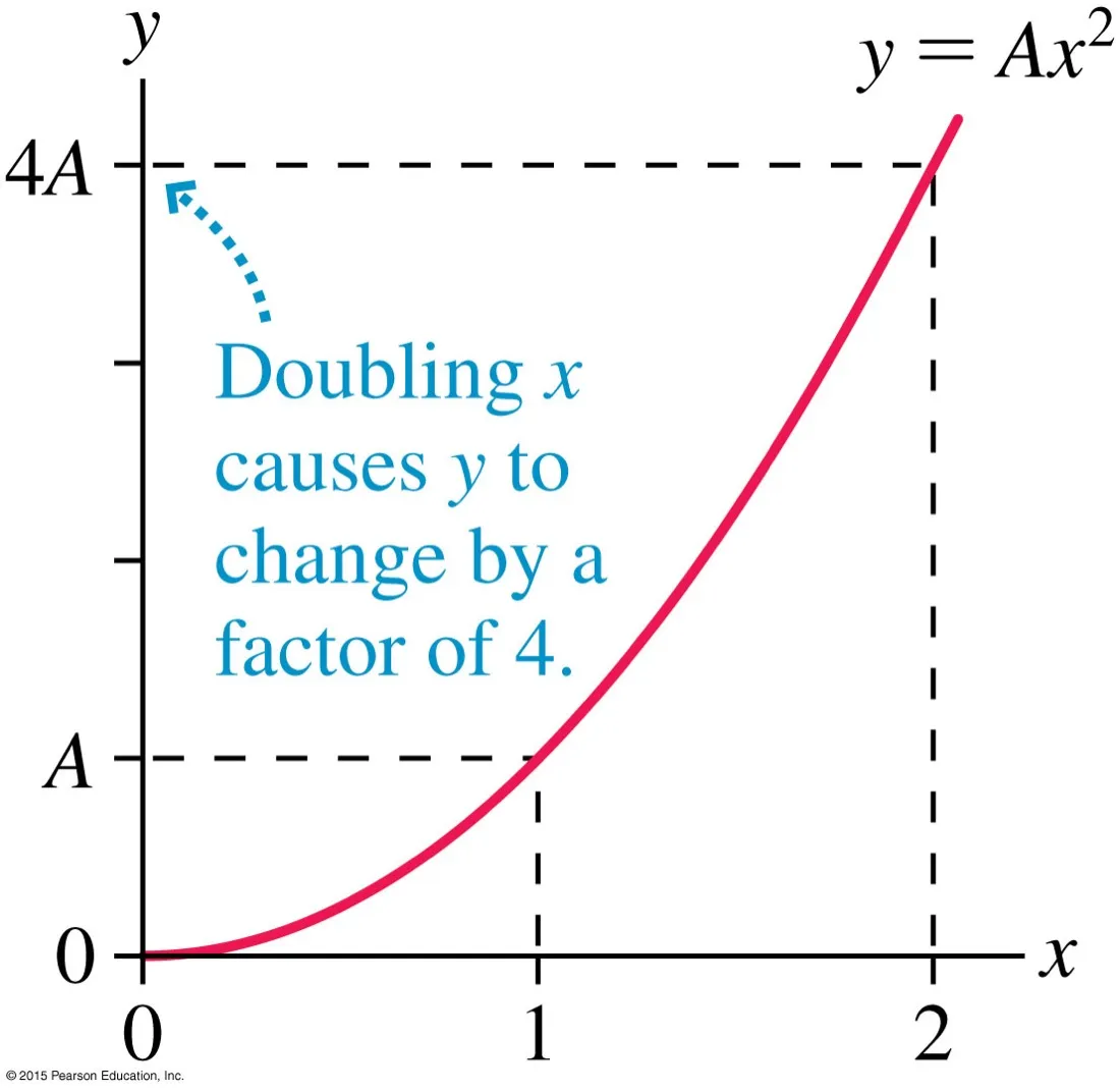
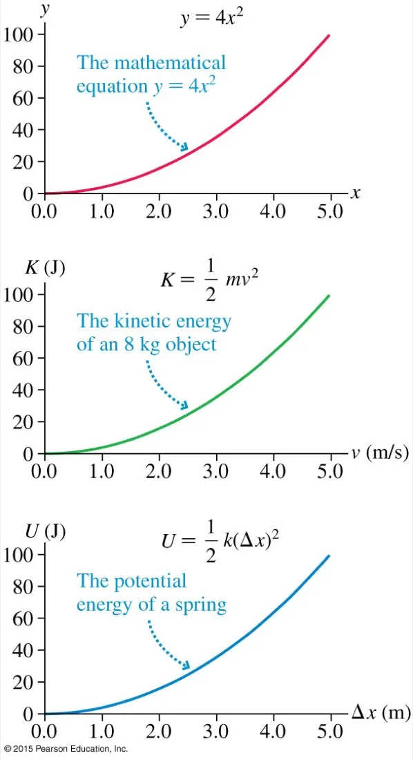
Constant velocity: area is a rectangle12 m s⁻¹ × 2 s = 24 m. The units multiply to metres, which is the check that the area really is a displacement and not just a number of grid squares.Changing velocity: area is a triangle½ × 3 s × 12 m s⁻¹ = 18 m. Not 12 × 3 — the object was slower than 12 m s⁻¹ for the entire interval except the final instant.Any shape at allThe rule does not need a straight line. For an awkward curve, count squares or split it into strips — the area is still the displacement, however you get at it.Where s = ut + ½at² comes fromRectangle uΔt plus triangle ½(aΔt)Δt. Add them and you have the second equation of motion. It is not something to memorise blindly — it is the area of this picture.The second shape pairStraight sloping v–t goes with parabolic x–t. Together with the constant-velocity pair, these two cover almost every graph you will be shown in A.1.Linear: double one, double the otherA straight line through the origin. In v = u + at from rest, doubling the time doubles the velocity. Recognising proportionality lets you answer some questions without any numbers at all.Quadratic: double one, quadruple the otherBecause s = ½at², doubling the fall time quadruples the distance fallen. Braking distance behaves the same way in v, which is why speed limits are not linear in their effect.One shape, three physics problemsIdentical curve, three meanings. Learning to recognise the shape rather than the context is what lets you carry kinematics into energy, fields and waves later on.
The concept students think they understand and consistently do not. The trap is the four-panel figure part way down — the one about what a negative acceleration actually means.
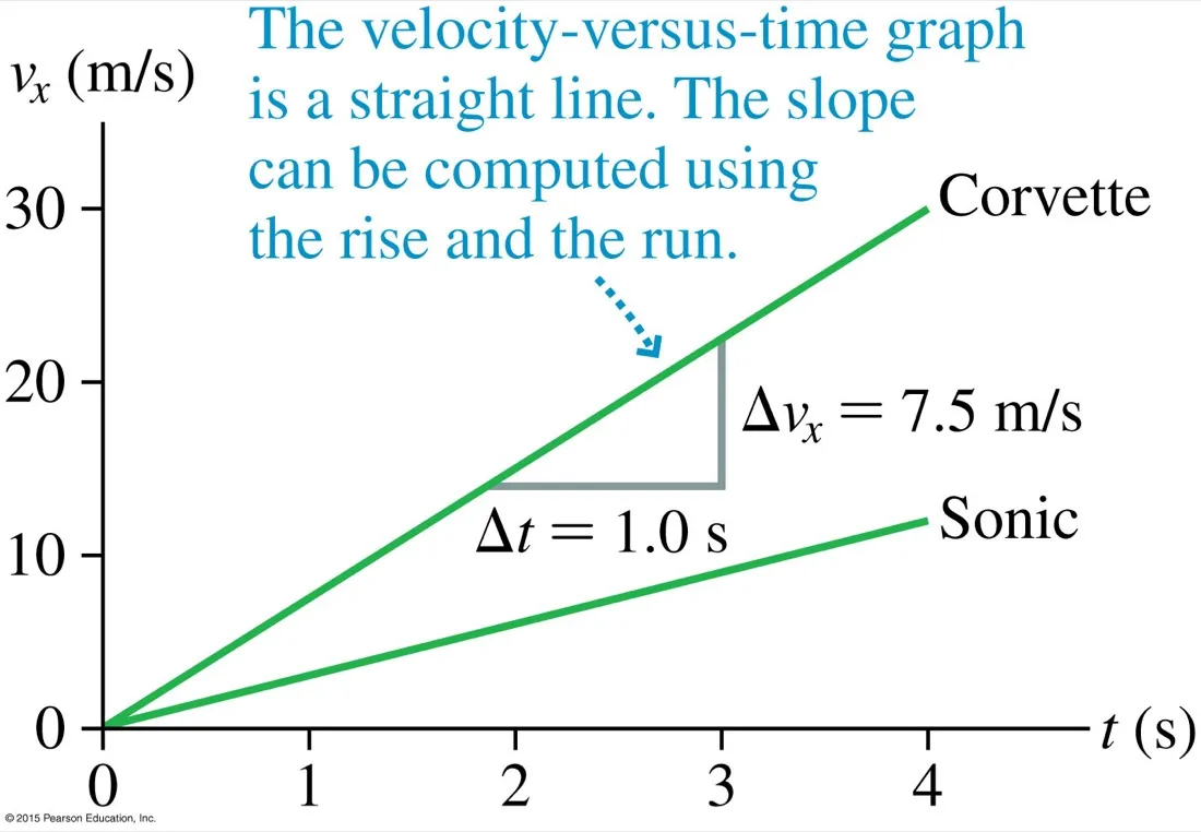
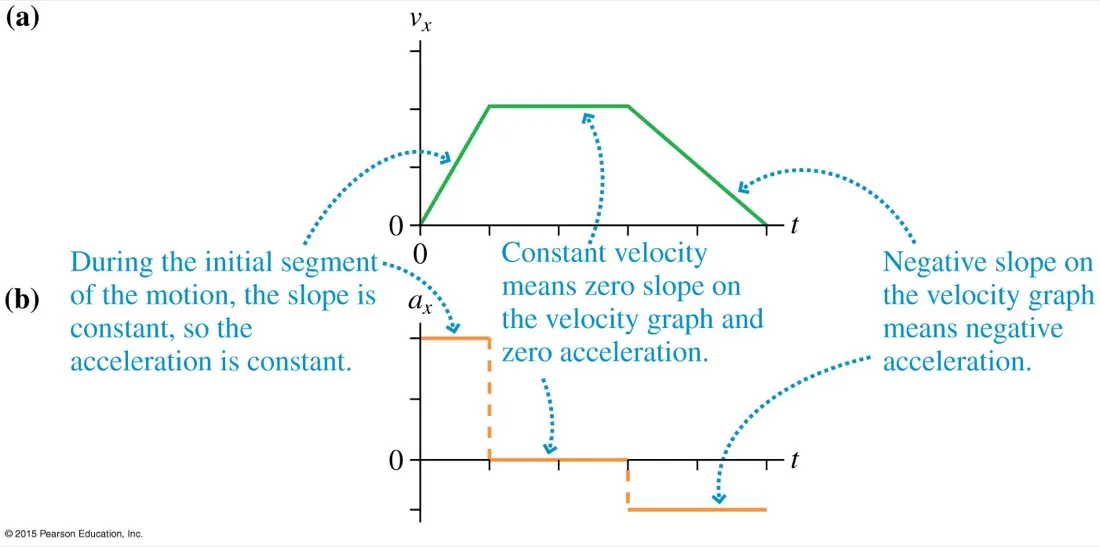
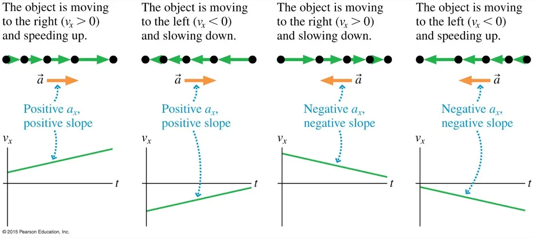
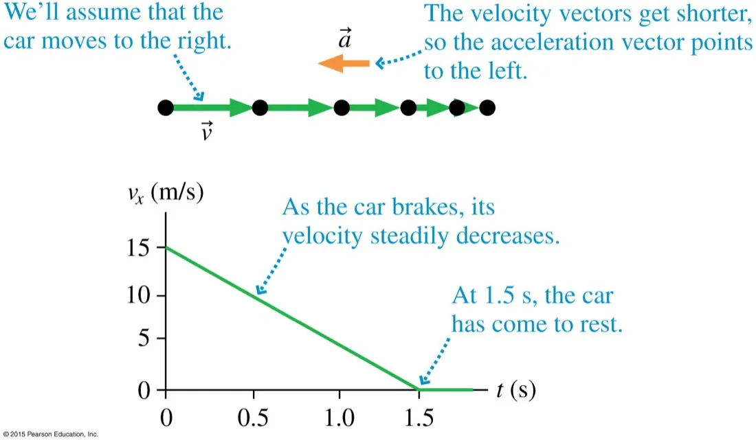
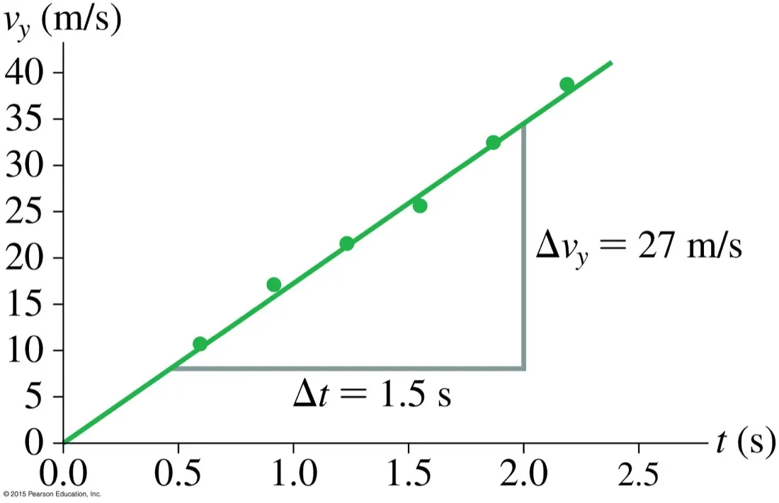
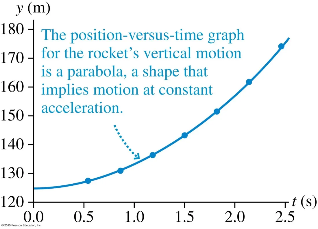
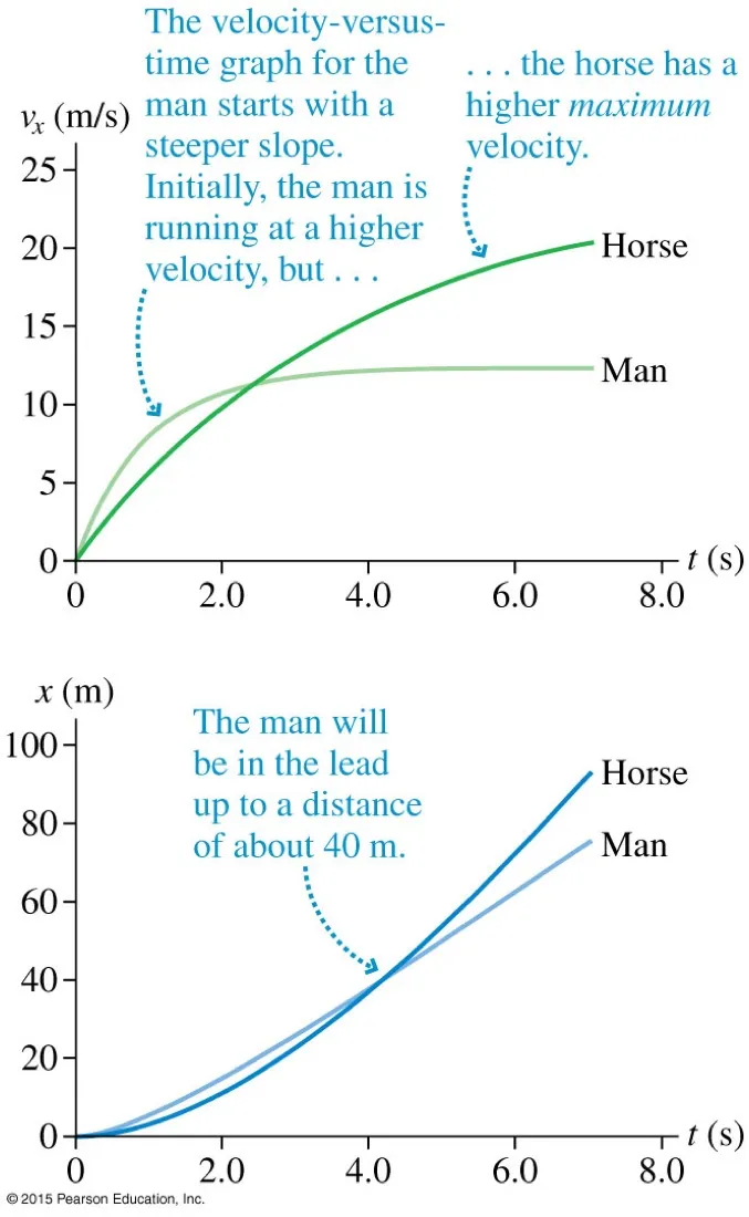
Both accelerating, not equallyBoth speed up; the Corvette's gaps grow faster. Acceleration is about how quickly the velocity changes, not how large the velocity is.Acceleration is the slope of v–t7.5 m s⁻¹ per second, written 7.5 m s⁻². The pattern repeats: slope of x–t is velocity, slope of v–t is acceleration. Same operation, one level down.Deriving a–t from v–tRising, flat, falling on v–t becomes positive, zero, negative on a–t. Constant velocity means zero acceleration — not constant acceleration, which is a common slip.The one to study hardestNegative acceleration does not mean slowing down. It means the acceleration points in the negative direction. Speeding up happens when a and v share a sign; slowing down when they oppose. Panel two — negative velocity, positive acceleration, slowing down — is the case that catches people.Braking, worked throughMoving right, so v is positive; slowing, so a is negative and the arrow points left. From 15 m s⁻¹ to 0 in 1.5 s gives a = −10 m s⁻². The car never reverses — the graph stops at zero.Acceleration from real dataThe points scatter; the line of best fit does not go through them all. 27 / 1.5 = 18 m s⁻². Take the gradient from the fitted line, never from two raw data points — that is the marked method.A parabola is a fingerprintCurved x–t means acceleration; a parabolicx–t means constant acceleration specifically, which is what licenses you to use the four equations.Higher acceleration, lower top speedThe man out-accelerates the horse and leads to about 40 m; the horse's higher maximum velocity wins after that. Two different quantities, two different winners — read which one the question is asking about.
Four equations, and a setup routine that matters more than the algebra.
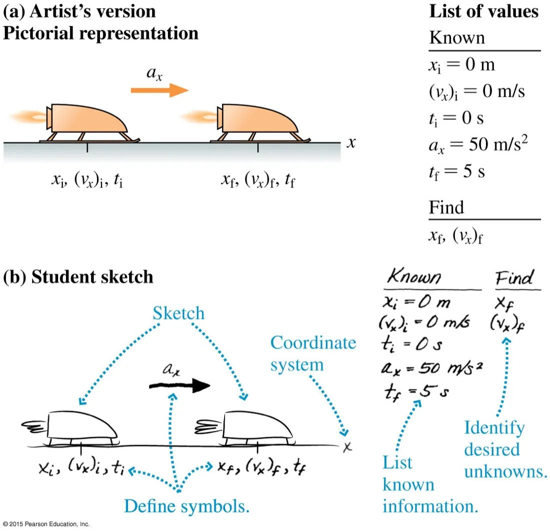
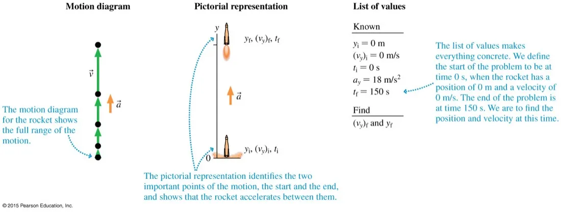
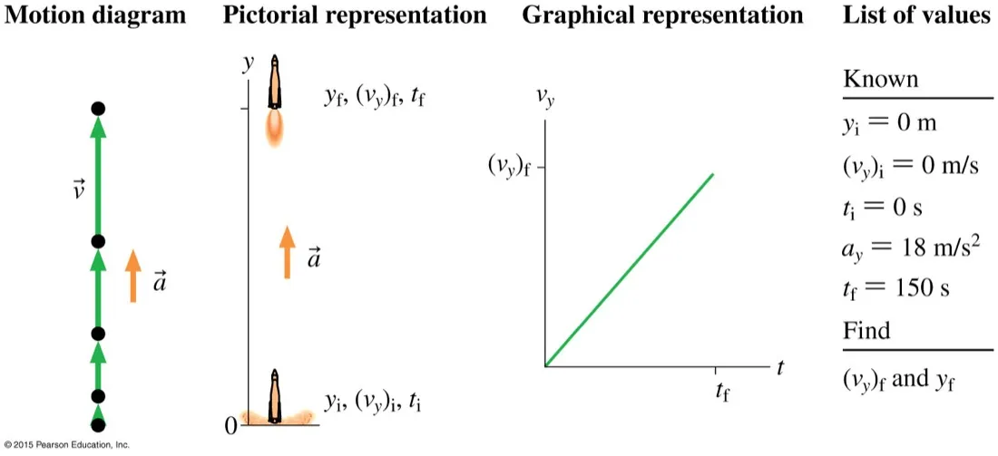
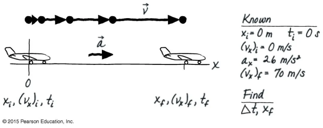
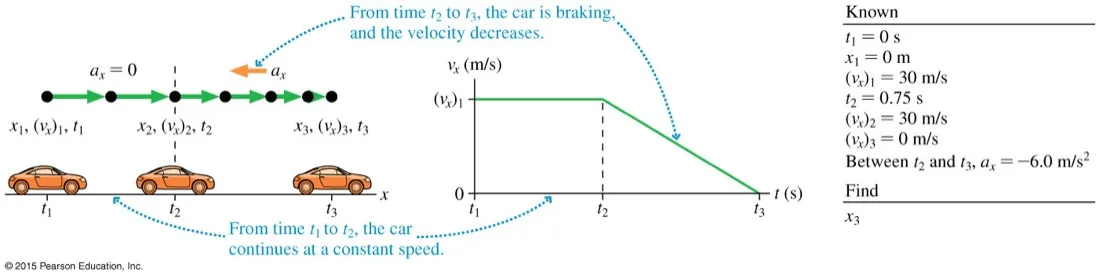
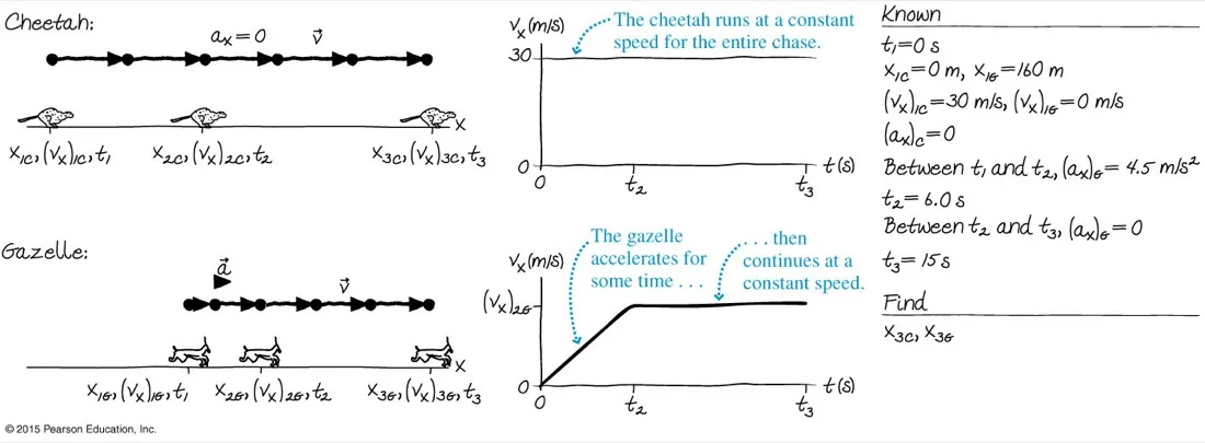
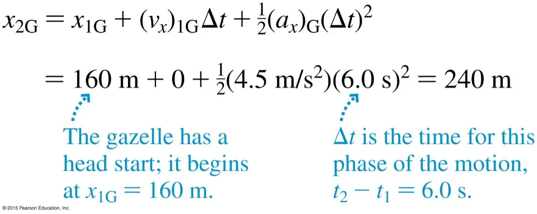
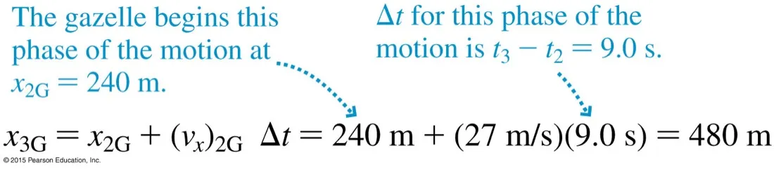
The setup that earns the marksSketch, axis, symbols, knowns, unknowns. The bottom version is what yours should look like — deliberately rough. Most failed kinematics problems fail here, not in the algebra.Three views of one problemMotion diagram for the shape of the motion, pictorial representation for the two states that matter, list of values for the algebra. Writing all three takes a minute and prevents most errors.Adding the graphThe same problem with a fourth view. If your algebra gives an answer your graph says is impossible, trust the graph and go back — it is far harder to draw a wrong graph than to make a sign error.What yours should look likeEntirely hand-drawn and perfectly adequate. Knowns on the right, unknowns named underneath. Notice xi = 0 and ti = 0 are choices made to simplify, not data from the question.Problems in phasesConstant speed to t₂, then braking to t₃. Apply the equations to each phase separately — they are only valid where the acceleration is constant. The end of one phase is the start of the next.Two objects, one clockThe hard part is bookkeeping, not physics. Subscript everything by object (C and G) and keep one shared time axis. The gazelle's 160 m head start is a difference in xi, nothing more.Phase one, in numbers160 m head start, starts from rest, accelerates at 4.5 m s⁻² for 6.0 s. Every symbol is subscripted so there is no doubt which animal it belongs to. Δt is the duration of this phase, not the total time.Phase two picks up where phase one stoppedThe 240 m from phase one becomes the starting position for phase two. Acceleration is now zero so the simpler equation applies. Chain the phases; never try to span both with one equation.
One acceleration, always the same, always downward — and the source of a great deal of confusion at the top of the flight.
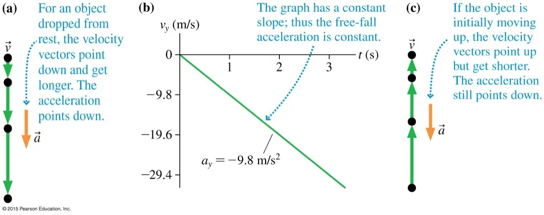
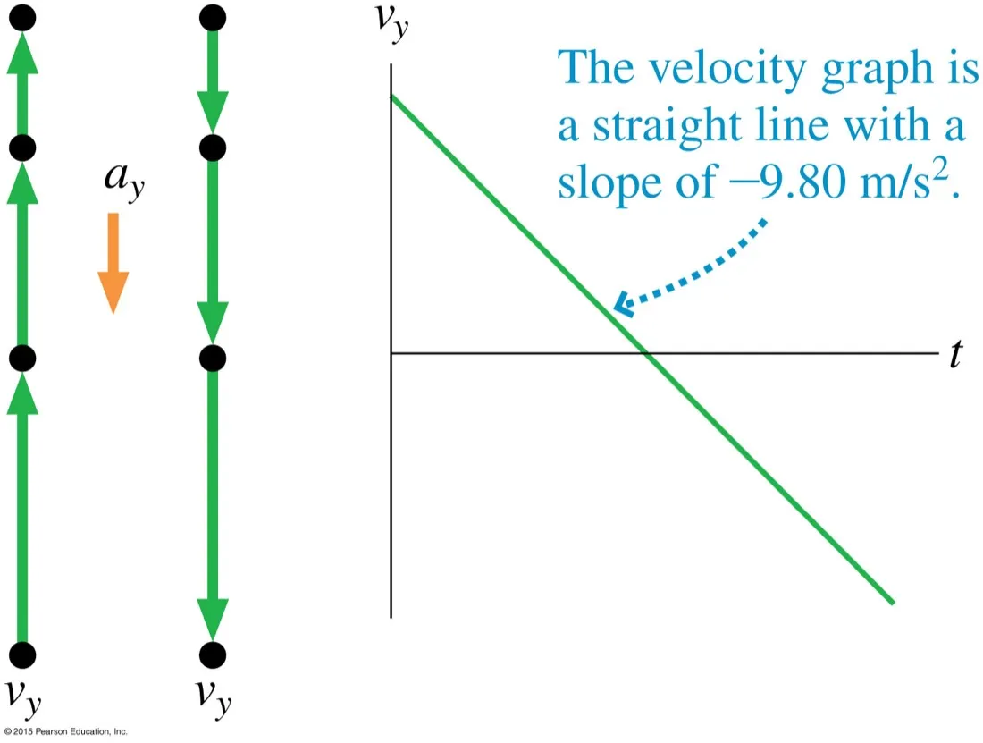
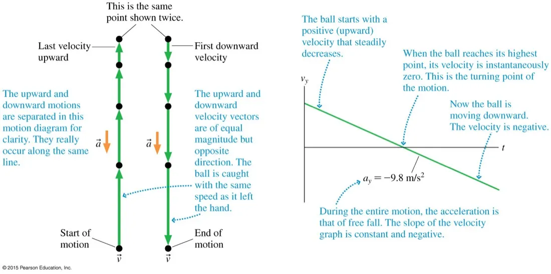
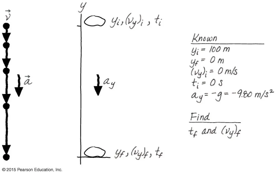
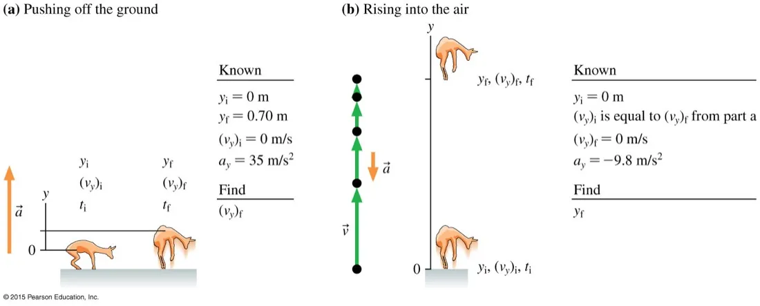
The acceleration never changesDropped or thrown upward, a = 9.8 m s⁻² downward throughout. Panel (c) is the one to sit with: the object is moving up while accelerating down. Nothing about that is contradictory.One straight line through zeroUp and down are not two problems. The v–t graph is a single straight line of slope −9.80 m s⁻² that happens to cross zero at the top. Treat the whole flight as one motion.At the top, v = 0 but a ≠ 0The two columns are drawn apart for clarity; the ball really goes straight up and back down the same line. At the highest point velocity is instantaneously zero while acceleration is still 9.8 m s⁻² down — if it were not, the ball would hang there.Setting up a fallAxis up, so the fall is from yi = 100 m to yf = 0 and ay = −9.80 m s⁻². Note g is written as a positive 9.80 and the minus comes from the direction — g itself is never negative.Free fall starts when contact endsWhile the legs are pushing, a = +35 m s⁻² and this is not free fall. The instant the feet leave the ground it becomes −9.8 m s⁻². The final velocity of phase one is the initial velocity of phase two.
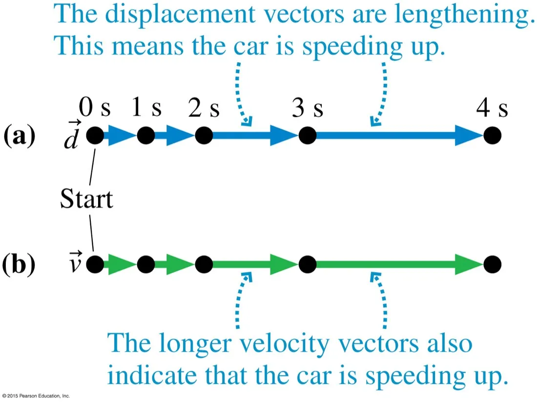
Two ways to draw the same thingDisplacement vectors span the gaps; velocity vectors do the same job scaled by 1/Δt. Both lengthen, both say speeding up. Knight uses velocity vectors from here on and so should you.Where A.1 goes in two dimensionsThe velocity vectors are tangent to the path and shortest at the top — the vertical component has gone while the horizontal one has not. That independence is the key to projectile motion.The tool you will need for itResolving into perpendicular components is what makes a projectile two independent one-dimensional problems. Everything on this page then applies twice — once horizontally, once vertically.